

|
CGAL 4.14 - 2D Polygon Partitioning
|
|
CGAL 4.14 - 2D Polygon Partitioning
|
A partition of a polygon \( P\) is a set of polygons such that the interiors of the polygons do not intersect and the union of the polygons is equal to the interior of the original polygon \( P\). This chapter describes functions for partitioning planar polygons into two types of subpolygons - \( y\)-monotone polygons and convex polygons. The partitions are produced without introducing new (Steiner) vertices.
All the partitioning functions present the same interface to the user. That is, the user provides a pair of input iterators, first and beyond, an output iterator result, and a traits class traits. The points in the range [first, beyond) are assumed to define a simple polygon whose vertices are in counterclockwise order. The computed partition polygons, whose vertices are also oriented counterclockwise, are written to the sequence starting at position result and the past-the-end iterator for the resulting sequence of polygons is returned. The traits classes for the functions specify the types of the input points and output polygons as well as a few other types and function objects that are required by the various algorithms.
A \( y\)-monotone polygon is a polygon whose vertices \( v_1, \ldots, v_n\) can be divided into two chains \( v_1, \ldots, v_k\) and \( v_k, \ldots, v_n, v_1\), such that any horizontal line intersects either chain at most once. For producing a \( y\)-monotone partition of a given polygon, the sweep-line algorithm presented in [1] is implemented by the function y_monotone_partition_2(). This algorithm runs in \( O(n \log n)\) time and requires \( O(n)\) space. This algorithm does not guarantee a bound on the number of polygons produced with respect to the optimal number.
For checking the validity of the partitions produced by y_monotone_partition_2(), we provide a function is_y_monotone_2(), which determines if a sequence of points in 2D defines a \( y\)-monotone polygon or not. For examples of the use of these functions, see the corresponding reference pages.
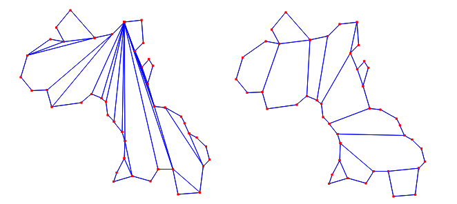
Three functions are provided for producing convex partitions of polygons. One produces a partition that is optimal in the number of pieces. The other two functions produce approximately optimal convex partitions. Both these functions produce convex decompositions by first decomposing the polygon into simpler polygons; the first uses a triangulation and the second a monotone partition. These two functions both guarantee that they will produce no more than four times the optimal number of convex pieces but they differ in their runtime complexities. Though the triangulation-based approximation algorithm often results in fewer convex pieces, this is not always the case.
An optimal convex partition can be produced using the function optimal_convex_partition_2().
This function provides an implementation of Greene's dynamic programming algorithm for optimal partitioning [2]. This algorithm requires \( O(n^4)\) time and \( O(n^3)\) space in the worst case.
The function approx_convex_partition_2() implements the simple approximation algorithm of Hertel and Mehlhorn [3] that produces a convex partitioning of a polygon from a triangulation by throwing out unnecessary triangulation edges. The triangulation used in this function is one produced by the 2-dimensional constrained triangulation package of CGAL. For a given triangulation, this convex partitioning algorithm requires \( O(n)\) time and space to construct a decomposition into no more than four times the optimal number of convex pieces.
The sweep-line approximation algorithm of Greene [2], which, given a monotone partition of a polygon, produces a convex partition in \( O(n \log n)\) time and \( O(n)\) space, is implemented by the function greene_approx_convex_partition_2(). The function y_monotone_partition_2() described in Section Monotone Partitioning is used to produce the monotone partition. This algorithm provides the same worst-case approximation guarantee as the algorithm of Hertel and Mehlhorn implemented with approx_convex_partition_2() but can sometimes produce better results (i.e., convex partitions with fewer pieces).
Examples of the uses of all of these functions are provided with the corresponding reference pages.
 1.8.13