

|
CGAL 4.6 - 2D and Surface Function Interpolation
|
|
CGAL 4.6 - 2D and Surface Function Interpolation
|
Scattered data interpolation solves the following problem: given measures of a function on a set of discrete data points, the task is to interpolate this function on an arbitrary query point.
If the function is a linear function and given barycentric coordinates that allow to express the query point as the convex combination of some data points, the function can be exactly interpolated. If the function gradients are known, we can exactly interpolate quadratic functions given barycentric coordinates. Any further properties of these interpolation functions depend on the properties of the barycentric coordinates. They are provided in this package under the name linear_interpolation() and quadratic_interpolation().
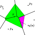
Natural neighbor coordinates are defined by Sibson in 1980 and are based on the Voronoi diagram of the data points. Interpolation methods based on natural neighbor coordinates are particularly interesting because they adapt easily to non-uniform and highly anisotropic data. This package contains Sibson's \( C^1\) continuous interpolation method which interpolates exactly spherical quadrics (of the form \( \Phi(\mathbf{x})=a + \mathbf{b}^t \mathbf{x} +\gamma\ \mathbf{x}^t\mathbf{x}\)) and Farin's \( C^1\) continuous interpolation method based on Bernstein-Bézier techniques and interpolating exactly quadratic functions - assuming that the function gradient is known. In addition, Sibson defines a method to approximate the function gradients for data points that are in the interior of the convex hull. This method is exact for spherical quadrics.
This CGAL package implements Sibson's and Farin's interpolation functions as well as Sibson's function gradient fitting method. Furthermore, it provides functions to compute the natural neighbor coordinates with respect to a two-dimensional Voronoi diagram (i. e., from the Delaunay triangulation of the data points) and to a two-dimensional power diagram for weighted points (i. e., from their regular triangulation). Natural neighbor coordinates on closed and well-sampled surfaces can also be computed if the normal to the surface at the query point is known. The latter coordinates are only approximately barycentric, see [2].
For a more thorough introduction see the user manual.
CGAL::linear_interpolationCGAL::sibson_c1_interpolationCGAL::farin_c1_interpolationCGAL::quadratic_interpolationCGAL::sibson_gradient_fittingCGAL::Interpolation_traits_2<K>CGAL::Interpolation_gradient_fitting_traits_2<K>CGAL::Voronoi_intersection_2_traits_3<K>CGAL::surface_neighbor_coordinates_3CGAL::surface_neighbors_3 Modules | |
| Concepts | |
| Interpolation Functions | |
| Natural Neighbor Coordinate Computation | |
| Surface Neighbor and Surface Neighbor Coordinate Computation | |
Classes | |
| struct | CGAL::Data_access< Map > |
The struct Data_access implements a functor that allows to retrieve data from an associative container. More... | |
 1.8.4
1.8.4