

|
CGAL 4.6 - 2D Minkowski Sums
|
|
CGAL 4.6 - 2D Minkowski Sums
|
Given two sets \( A,B \in \mathbb{R}^d\), their Minkowski sum, denoted by \( A \oplus B\), is the set \( \left\{ a + b ~|~ a \in A, b \in B \right\}\). Minkowski sums are used in many applications, such as motion planning and computer-aided design and manufacturing. This package contains functions for computing planar Minkowski sums of two polygons (namely \( A\) and \( B\) are two closed polygons in \( \mathbb{R}^2\)), and for a polygon and a disc (an operation also known as offsetting or dilating a polygon).
Computing the Minkowski sum of two convex polygons \( P\) and \( Q\) with \( m\) and \( n\) vertices respectively is very easy, as \( P \oplus Q\) is a convex polygon bounded by copies of the \( m + n\) edges, and these edges are sorted by the angle they form with the \( x\)-axis. As the two input polygons are convex, their edges are already sorted by the angle they form with the \( x\)-axis. The Minkowski sum can therefore be computed in \( O(m + n)\) time, by starting from two bottommost vertices in \( P\) and in \( Q\) and performing "merge sort" on the edges.
| 
|
If the polygons are not convex, it is possible to use one of the following approaches:
We decompose \( P\) and \( Q\) into convex sub-polygons, namely we obtain two sets of convex polygons \( P_1, \ldots, P_k\) and \( Q_1, \ldots, Q_\ell\) such that \( \bigcup_{i = 1}^{k}{P_i} = P\) and \( \bigcup_{i = j}^{\ell}{Q_j} = Q\). We then calculate the pairwise sums \( S_{ij} = P_i \oplus Q_j\) using the simple procedure described above, and compute the union \( P \oplus Q = \bigcup_{ij}{S_{ij}}\).
This approach relies on a decomposition strategy that computes the convex decomposition of the input polygons and its performance depends on the quality of the decomposition.
Let us denote the vertices of the input polygons by \( P = \left( p_0, \ldots, p_{m-1} \right)\) and \( Q = \left( q_0, \ldots, q_{n-1} \right)\). We assume that both \( P\) and \( Q\) have positive orientations (i.e. their boundaries wind in a counterclockwise order around their interiors) and compute the convolution of the two polygon boundaries. The convolution of these two polygons [5], denoted \( P * Q\), is a collection of line segments of the form \( [p_i + q_j, p_{i+1} + q_j]\), Throughout this chapter, we increment or decrement an index of a vertex modulo the size of the polygon. where the vector \( {\mathbf{p_i p_{i+1}}}\) lies between \( {\mathbf{q_{j-1} q_j}}\) and \( {\mathbf{q_j q_{j+1}}}\), We say that a vector \( {\mathbf v}\) lies between two vectors \( {\mathbf u}\) and \( {\mathbf w}\) if we reach \( {\mathbf v}\) strictly before reaching \( {\mathbf w}\) if we move all three vectors to the origin and rotate \( {\mathbf u}\) counterclockwise. Note that this also covers the case where \( {\mathbf u}\) has the same direction as \( {\mathbf v}\). and, symmetrically, of segments of the form \( [p_i + q_j, p_i + q_{j+1}]\), where the vector \( {\mathbf{q_j q_{j+1}}}\) lies between \( {\mathbf{p_{i-1} p_i}}\) and \( {\mathbf{p_i p_{i+1}}}\).
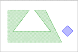
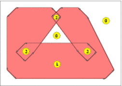
The segments of the convolution form a number of closed (not necessarily simple) polygonal curves called convolution cycles. The Minkowski sum \( P \oplus Q\) is the set of points having a non-zero winding number with respect to the cycles of \( P * Q\). Informally speaking, the winding number of a point \( p \in\mathbb{R}^2\) with respect to some planar curve \( \gamma\) is an integer number counting how many times does \( \gamma\) wind in a counterclockwise direction around \( p\). See Figure 21.1 for an illustration.
The number of segments in the convolution of two polygons is usually smaller than the number of segments that constitute the boundaries of the sub-sums \( S_{ij}\) when using the decomposition approach. As both approaches construct the arrangement of these segments and extract the sum from this arrangement, computing Minkowski sum using the convolution approach usually generates a smaller intermediate arrangement, hence it is faster and consumes less space.
The function minkowski_sum_2(P, Q) accepts two simple polygons \( P\) and \( Q\), represented using the Polygon_2<Kernel,Container> class-template and uses the convolution method in order to compute and return their Minkowski sum \( S = P \oplus Q\).
As the input polygons may not be convex, their Minkowski sum may not be simply connected and contain polygonal holes; see for example Figure 21.1. \( S\) is therefore an instance of the Polygon_with_holes_2<Kernel,Container> class-template, defined in the Boolean Set-Operations package: The outer boundary of \( S\) is a polygon that can be accessed using S.outer_boundary(), and its polygonal holes are given by the range [S.holes_begin(), S.holes_end()) (where \( S\) contains S.number_of_holes() holes in its interior).
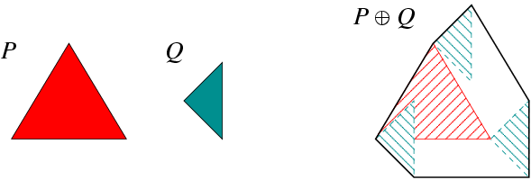
The following example program constructs the Minkowski sum of two triangles, as depicted in Figure 21.2. The result in this case is a convex hexagon. This program, as other example programs in this chapter, includes the auxiliary header file ms_rational_nt.h which defines Number_type as either Gmpq or Quotient<MP_Float>, depending on whether the Gmp library is installed or not. The file print_util.h includes auxiliary functions for printing polygons.
File Minkowski_sum_2/sum_triangles.cpp
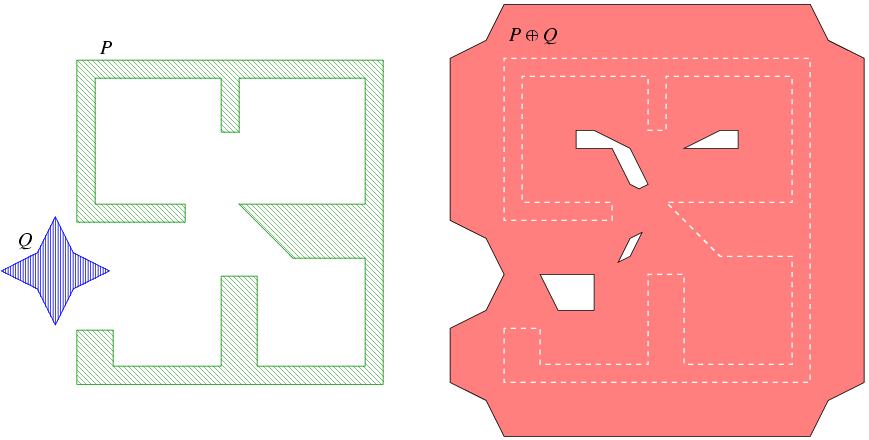
In the following program we compute the Minkowski sum of two polygons that are read from an input file. In this case, the sum is not simple and contains four holes, as illustrated in Figure 21.3. Note that this example uses the predefined CGAL kernel with exact constructions. In general, instantiating polygons with this kernel yields the fastest running times for Minkowski-sum computations.
File Minkowski_sum_2/sum_with_holes.cpp
In order to compute Minkowski sums using the decomposition method, it is possible to call the function minkowski_sum_2(P, Q, decomp), where decomp is an instance of a class that models the concept PolygonConvexDecomposition_2, namely it should provide a method named decompose() that receives a planar polygon and returns a range of convex polygons that represents its convex decomposition.
The Minkowski-sum package includes four models of the concept PolygonConvexDecomposition_2. The first three are classes that wrap the decomposition functions included in the Planar Polygon Partitioning package, while the fourth is an implementation of a decomposition algorithm introduced in [1]. The convex decompositions that it creates usually yield efficient running times for Minkowski sum computations:
Optimal_convex_decomposition_2<Kernel> uses the dynamic-programming algorithm of Greene [4] for computing an optimal decomposition of a polygon into a minimal number of convex sub-polygons. The main drawback of this strategy is that it runs in \( O(n^4)\) time and \( O(n^3)\) in the worst case,where \( n\) is the number of vertices in the input polygon. Hertel_Mehlhorn_convex_decomposition_2<Kernel> implements the approximation algorithm suggested by Hertel and Mehlhorn [6], which triangulates the input polygon and proceeds by throwing away unnecessary triangulation edges. This algorithm requires \( O(n)\) time and space and guarantees that the number of sub-polygons it generates is not more than four times the optimum. Greene_convex_decomposition_2<Kernel> is an implementation of Greene's approximation algorithm [4], which computes a convex decomposition of the polygon based on its partitioning into \( y\)-monotone polygons. This algorithm runs in \( O(n \log n)\) time and \( O(n)\) space, and has the same approximation guarantee as Hertel and Mehlhorn's algorithm. Small_side_angle_bisector_decomposition_2<Kernel> uses a heuristic improvement to the angle-bisector decomposition method suggested by Chazelle and Dobkin [2], which runs in \( O(n^2)\) time. It starts by examining each pair of reflex vertices in the input polygon such that the entire interior of the diagonal connecting these vertices is contained in the polygon. Out of all available pairs, the vertices \( p_i\) and \( p_j\) are selected such that the number of reflex vertices from \( p_i\) to \( p_j\) (or from \( p_j\) to \( p_i\)) is minimal. The polygon is split by the diagonal \( p_i p_j\) and we continue recursively on both resulting sub-polygons. In case it is not possible to eliminate two reflex vertices at once any more, each reflex vertex is eliminated by a diagonal that is closest to the angle bisector emanating from this vertex. The following example demonstrates the computation of the Minkowski sum of the same input polygons as used in Minkowski_sum_2/sum_with_holes.cpp (as depicted in Figure 21.3), using the small-side angle-bisector decomposition strategy:
File Minkowski_sum_2/sum_by_decomposition.cpp
The operation of computing the Minkowski sum \( P \oplus B_r\) of a polygon \( P\) with \( b_r\), a disc of radius \( r\) centered at the origin, is widely known as offsetting the polygon \( P\) by a radius \( r\).
| 
| 
|
| (a) | (b) | (c) |
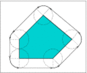
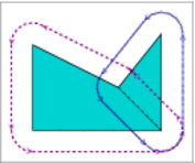
Let \( P = \left( p_0, \ldots, p_{n - 1} \right)\) be the polygon vertices, ordered in a counterclockwise orientation around its interior. If \( P\) is a convex polygon the offset is easily computed by shifting each polygon edge by \( r\) away from the polygon, namely to the right side of the edge. As a result we obtain a collection of \( n\) disconnected offset edges. Each pair of adjacent offset edges, induced by \( p_{i-1} p_i\) and \( p_i p_{i+1}\), are connected by a circular arc of radius \( r\), whose supporting circle is centered at \( p_i\). The angle that defines such a circular arc equals \( 180^{\circ} - \angle (p_{i-1}, p_i, p_{i+1})\); see Figure 21.4 (a) for an illustration. The running time of this simple process is of course linear with respect to the size of the polygon.
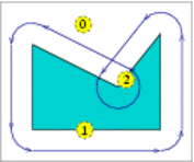
If \( P\) is not convex, its offset can be obtained by decomposing it to convex sub-polygons \( P_1, \ldots P_m\) such that \( \bigcup_{i=1}^{m}{P_i} = P\), computing the offset of each sub-polygon and finally calculating the union of these sub-offsets (see Figure 21.4 (b)). However, as was the case with the Minkowski sum of a pair of polygons, here it is also more efficient to compute the convolution cycle of the polygon with the disc \( B_r\), As the disc is convex, it is guaranteed that the convolution curve is comprised of a single cycle. which can be constructed by applying the process described in the previous paragraph. The only difference is that a circular arc induced by a reflex vertex \( p_i\) is defined by an angle \( 540^{\circ} - \angle (p_{i-1}, p_i, p_{i+1})\); see Figure 21.4 (c) for an illustration. We finally compute the winding numbers of the faces of the arrangement induced by the convolution cycle to obtain the offset polygon.
Let us assume that we are given a counterclockwise-oriented polygon \( P = \left( p_0, \ldots, p_{n-1} \right)\), whose vertices all have rational coordinates (i.e., for each vertex \( p_i = (x_i, y_i)\) we have \( x_i, y_i \in {\mathbb Q}\), and we wish to compute its Minkowski sum with a disc of radius \( r\), where \( r\) is also a rational number. The boundary of this sum is comprised of line segments and circular arcs, where:
\[ \frac{(ax + by + c)^2}{a^2 + b^2} = r^2 \ . \]
Thus, the linear offset edges are segments of curves of an algebraic curve of degree 2 (a conic curve) with rational coefficients. This curve is actually a pair of the parallel lines \( ax + by + (c \pm \ell\cdot r) = 0\). In Section Computing the Exact Offset we use this representation to construct the offset polygon in an exact manner using the traits class for conic arcs.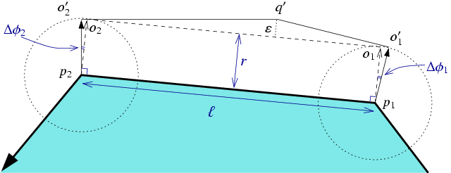
The class-template Gps_circle_segment_traits_2<Kernel>, included in the Boolean Set-Operations package is used for representing general polygons whose edges are circular arcs or line segments, and for applying set operations (e.g. intersection, union, etc.) on such general polygon. It should be instantiated with a geometric kernel that employs exact rational arithmetic, such that the curves that comprise the polygon edges should be arcs of circles with rational coefficients or segments of lines with rational coefficients. As in our case the line segments do not satisfy this requirement, we apply a simple approximation scheme, such that each irrational line segment is approximated by two rational segments:
The function approximated_offset_2(P, r, eps) accepts a polygon \( P\), an offset radius \( r\) and \( \varepsilon > 0\). It constructs an approximation for the offset of \( P\) by the radius \( r\) using the procedure explained above. Furthermore, it is guaranteed that the approximation error, namely the distance of the point \( q'\) from \( o_1 o_2\) is bounded by \( \varepsilon\). Using this function, we are capable of working with the Gps_circle_segment_traits_2<Kernel> class, which considerably speeds up the (approximate) construction of the offset polygon and the application of set operations on such polygons. The function returns an object of the nested type Gps_circle_segment_traits_2::Polygon_with_holes_2 representing the approximated offset polygon (recall that if \( P\) is not convex, its offset may not be simple and may contain holes, whose boundary is also comprised of line segments and circular arcs).
The following example demonstrates the construction of an approximated offset of a non-convex polygon, as depicted in Figure 21.6. Note that we use a geometric kernel parameterized with a filtered rational number-type. Using filtering considerably speeds up the construction of the offset.
File Minkowski_sum_2/approx_offset.cpp
As we previously mentioned, it is possible to represent offset polygons in an exact manner, if we treat their edges as arcs of conic curves with rational coefficients. The function offset_polygon_2(P, r, traits) computes the offset of the polygon \( P\) by a rational radius \( r\) in an exact manner. The traits parameter should be an instance of an arrangement-traits class that is capable of handling conic arcs in an exact manner; using the Arr_conic_traits_2 class with the number types provided by the Core library is the preferred option. The function returns an object of the nested type Gps_traits_2::Polygons_with_holes_2 (see the documentation of the Boolean Set-Operations package for more details on the traits-class adapter Gps_traits_2), which represented the exact offset polygon.
The following example demonstrates the construction of the offset of the same polygon that serves as an input for the example program Minkowski_sum_2/approx_offset.cpp, presented in the previous subsection (see also Figure 21.6). Note that the resulting polygon is smaller than the one generated by the approximated-offset function (recall that each irrational line segment in this case is approximated by two rational line segments), but the offset computation is considerably slower:
File Minkowski_sum_2/exact_offset.cpp
Both functions approximated_offset_2() and offset_polygon_2() also have overloaded versions that accept a decomposition strategy and use the polygon-decomposition approach to compute (or approximate) the offset. These functions are less efficient than their counterparts that employ the convolution approach, and are only included in the package for the sake of completeness.
An operation closely related to the offset computation, is obtaining the inner offset of a polygon, or insetting it by a given radius. The inset of a polygon \( P\) with radius \( r\) is the set of points iside \( P\) whose distance from the polygon boundary, denoted \( \partial P\), is at least \( r\) - namely: \( \{ p \in P \;|\; {\rm dist}(p, \partial P) \geq r \}\). Note that the resulting set may not be connected in case \( P\) is a non-convex polygon that has some narrow components, and thus is characterized by a (possibly empty) set of polygons whose edges are line segments and circular arcs of radius \( r\).
The offset can be computed using the convolution method if we traverse the polygon in a clockwise orientation (and not in counterclockwise orientation, as done in case of ofsetting a polygon). As in case of the offset functions, the Minkowski-sum package contains two functions for insetting a simple polygon:
The function approximated_inset_2(P, r, eps, oi) accepts a polygon \( P\), an inset radius \( r\) and \( \varepsilon > 0\). It constructs an approximation for the inset of \( P\) by the radius \( r\), with the approximation error bounded by \( \varepsilon\). The function returns its output via the output iterator oi, whose value-type must be Gps_circle_segment_traits_2::Polygon_2 representing the polygons that approximates the inset polygon.
File Minkowski_sum_2/approx_inset.cpp
Similarly, the function inset_polygon_2(P, r, traits, oi) computes the exact inset of \( P\) with radius \( r\), and returns its output via the given output iterator oi. The traits parameter should be an instance of an arrangement-traits class that is capable of handling conic arcs in an exact manner, whereas oi's value-type must be Gps_traits_2::Polygon_2.
File Minkowski_sum_2/exact_inset.cpp
Unlike the offset functions, there are no overloaded versions of the inset functions that use convex polygon decomposition to compute insets, as this method cannot be easily generalized for inset computations.
In this context let us mention that there exist overloaded versions of the functions approximated_offset_2(P, r, eps) and offset_polygon_2(P, r, traits) that accept a polygon with holes \( P\) and computed its offset. This ofset is obtain by taking the outer offset of \( P\)'s outer boundary, and computing the inner offsets of \( P\)'s holes. The former polygon defines the output boundary of \( P \oplus B_r\), and the latter define the holes within the result.
Andreas Fabri and Laurent Rineau helped tracing and solving several bugs in the approximated offset function. They have also suggested a few algorithmic improvements that made their way into version 3.4, yielding a faster approximation scheme.
 1.8.4
1.8.4