|
CGAL 4.8.1 - Point Set Shape Detection
|
|
CGAL 4.8.1 - Point Set Shape Detection
|
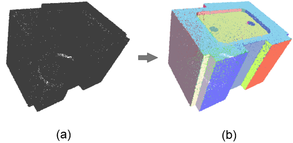
This CGAL component implements the efficient RANSAC method for shape detection, contributed by Schnabel et al. [1]. From an unstructured point set with unoriented normals, the algorithm detects a set of shapes (see Figure 69.1). Five types of primitive shapes are provided by this package: plane, sphere, cylinder, cone and torus. Detecting other types of shapes requires implementing a class derived from a base shape.

The method takes as input a point set with unoriented normals and provides as output a set of detected shapes with associated input points. The shapes are detected via a RANSAC-type approach, i.e., a random sample consensus. The basic RANSAC approach repeats the following steps: (1) Randomly select samples from the input points. (2) Fit a shape to the selected samples. (3) Count the number of inliers to the shape, inliers being within a user-specified error tolerance to the shape. Steps 1-3 are repeated for a prescribed number of iterations and the shape with highest number of inliers, referred to as largest shape, is kept.
In our context, the error between a point and a shape is defined by its distance and normal deviation to the shape. A random subset corresponds to the minimal number of points (with normals) required to uniquely define a primitive.
For very large point sets the basic RANSAC method is not practical when testing all possible shape candidates against the input data in order to find the largest shape. The main idea behind the efficient RANSAC method consists in testing shape candidates against subsets of the input data. Shape candidates are constructed until the probability to miss the largest candidate is lower than a user-specified parameter. The largest shape is repeatedly extracted until no more shapes, restricted to cover a minimum number of points, can be extracted. An additional gain in efficiency is achieved through exploiting the normal attributes during initial shape construction and enumeration of inliers.
The support of a shape refers to the footprint of the points covered by the primitive. To avoid generating shapes with fragmented support we enforce a connectivity constraint by considering only one connected component, referred to as cluster, selected as the one covering the largest number of inliers. See Section Parameters for more details.
The output of the shape detection algorithm is a set of detected shapes with assigned points, and all remaining points not covered by shapes. Each input point can be assigned to at most one detected shape.
The algorithm has five parameters:
epsilon and normal_threshold: The error between a point-with-normal \(p\) and a shape \(S\) is defined by its Euclidean distance and normal deviation to \(S\). The normal deviation is computed between the normal at \(p\) and the normal of \(S\) at the closest projection of \(p\) onto \(S\). Parameter epsilon defines the absolute maximum tolerance Euclidean distance between a point and a shape. A high value for epsilon leads to the detection of fewer large shapes and hence a less detailed detection. A low value for epsilon yields a more detailed detection, but may lead to either lower coverage or over-segmentation. Over-segmentation translates into detection of fragmented shapes when epsilon is within or below the noise level. When the input point set is made of free-form parts, a higher tolerance epsilon allows for detecting more primitive shapes that approximate some of the free-form surfaces. The impact of this parameter is depicted by Figure Figure 69.2. Its impact on performance is evaluated in Section Performance. 
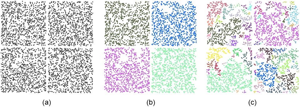
cluster_epsilon: Clustering of the points into connected components covered by a detected shape is controlled via parameter cluster_epsilon. For developable shapes that admit a trivial planar parameterization (plane, cylinder, cone) the points covered by a shape are mapped to a 2D parameter space chosen to minimize distortion and best preserve arc-length distances. This 2D parameter space is discretized using a regular grid, and a connected component search is performed to identify the largest cluster. Parameter cluster_epsilon defines the spacing between two cells of the regular grid, so that two points separated by a distance of at most \(2\sqrt{2}\), cluster_epsilon are considered adjacent. For non-developable shapes the connected components are identified by computing a neighboring graph in 3D and walking in the graph. The impact of parameter cluster_epsilon is depicted by Figure Figure 69.3. 
probability: This parameter defines the probability to miss the largest candidate shape. A lower probability provides a higher reliability and determinism at the cost of longer running times due to higher search endurance.min_points: This minimum number of points controls the termination of the algorithm. The shape search is iterated until no further shapes can be found with a higher support. Note that this parameter is not strict: depending on the chosen probability, shapes may be extracted with a number of points lower than the specified parameter.The main class Shape_detection_3::Efficient_RANSAC takes a template parameter Shape_detection_3::Efficient_RANSAC_traits that defines the geometric types and input format. Property maps provide a means to interface with user-specific data structures. The first parameter of the Shape_detection_3::Efficient_RANSAC_traits class is the common Kernel. In order to match the constraints of property maps, an iterator type and two maps that map an iterator to a point and a normal are specified in the Shape_detection_3::Efficient_RANSAC_traits class. The concept behind property maps is detailed in a dedicated chapter.
Typical usage consists in five steps:
The following minimal example reads a point set from a file and detects only planar shapes. The default parameters are used for detection.
File Point_set_shape_detection_3/efficient_RANSAC_basic.cpp
This example illustrates the user selection of parameters using the Shape_detection_3::Efficient_RANSAC::Parameters struct. Shape detection is performed on five types of shapes (plane, cylinder, sphere, cone, torus). Basic information of the detected shapes is written to the standard output. The input point set is sampled on a surface mostly composed of piece-wise planar and cylindrical parts, in addition to free-form parts.
File Point_set_shape_detection_3/efficient_RANSAC_parameters.cpp
This example illustrates how to access the points assigned to each shape and compute the mean error. A timer measures the running performance.
File Point_set_shape_detection_3/efficient_RANSAC_point_access.cpp
Other types of shapes can be detected by implementing a shape class derived from the class Shape_base and registering it to the shape detection factory. This class must provide the following functions: construct a shape from a small set of given points, compute the squared distance from a query point and the shape and compute the normal deviation between a query point with normal and the normal to the shape at the closest point from the query. The used shape parameters are added as members to the derived class.
Note that the RANSAC approach is efficient for shapes that are uniquely defined by a small number of points, denoted by the number of required samples. The algorithm aims at detected the largest shape via many random samples, and the combinatorial complexity of possible samples increases rapidly with the number of required samples.
More specifically, the functions to be implemented are defined in the base class Shape_detection_3::Shape_base:
Shape_detection_3::Shape_base::minimum_sample_size() const: Returns the minimal number of required samples.Shape_detection_3::Shape_base::create_shape(const std::vector<size_t> &indices): The randomly generated samples are provided via a vector of indices. Shape_detection_3::Shape_base::point(size_t i) and Shape_detection_3::Shape_base::normal(size_t i) are used to retrieve the actual points and normals (see example below). The provided number of samples might actually be larger than the set minimal number of required samples, depending on the other types of shape types. If the provided samples are not sufficient for define a unique shape, e.g., in a degenerated case the shape is considered invalid.Shape_detection_3::Shape_base::squared_distance(const Point &p) const: This function computes the squared distance from a query point to the shape. It is used for traversing the hierarchical spatial data structure.Shape_detection_3::Shape_base::squared_distance(std::vector<FT> &dists, const std::vector<size_t> &indices)Shape_detection_3::Shape_base::cos_to_normal(const std::vector<size_t> &indice, sstd::vector<FT> &angles) const: These functions are used to determine the number of inlier points to the shape. They compute respectively the squared distance from a set of points to the shape, and the dot product between the point's normals and the normals at the shape for the closest points on the shape. The access to the actual point and normal data is carried out via Shape_detection_3::Shape_base::point(size_t i) and Shape_detection_3::Shape_base::normal(size_t i) (see example below). The resulting squared distance/dot product is stored in the vector provided as the first argument.By default the connected component is detected via the neighbor graph as mentioned above. However, for shapes that admit a faster approach to detect a connected component, the user can provide his/her own implementation to extract the connected component via:
Shape_detection_3::Shape_base::connected_component(std::vector<std::size_t>& indices, FT cluster_epsilon): The indices of all supporting points are stored in the vector indices. All points not belonging to the largest cluster of points are removed from the vector indices.Another optional method can be implemented to provide a helper function providing the shape parameters written to a string:
Shape_detection_3::Shape_base::info(): This function returns a string suitable for printing the shape parameters into a log/console. The default solution provides an empty string.The property maps are used to map the indices to the corresponding points and normals. The following example shows an implementation of a planar shape primitive, which is used by the example Point_set_shape_detection_3/efficient_RANSAC_custom_shape.cpp.
File Point_set_shape_detection_3/efficient_RANSAC_custom_shape.h
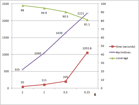
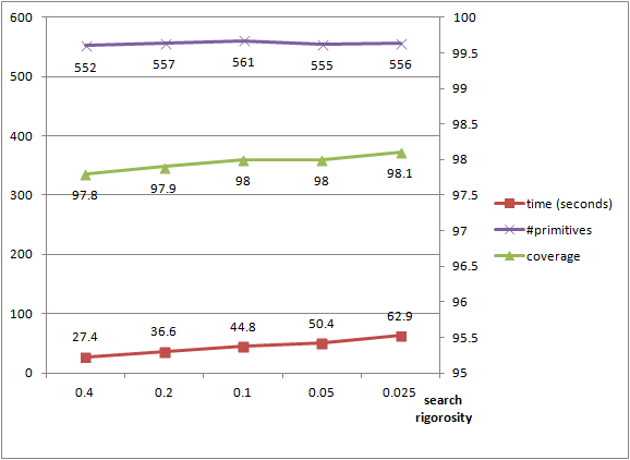
The running time and detection performance depend on the chosen parameters. A selective error tolerance parameter leads to higher running times and smaller shapes, as many shape candidates are generated to find the largest shape. We plot the detection performance against the epsilon error tolerance parameter for detecting planes in a complex scene with 5M points, see Figure 69.4. The probability parameter controls the endurance when searching for the largest candidate at each iteration. It barely impacts the number of detected shapes, has a moderate impact on the size of the detected shapes and increases the running times. We plot the performance against the probability parameter, see Figure 69.5.

