

|
CGAL 4.8.2 - Linear and Quadratic Programming Solver
|
|
CGAL 4.8.2 - Linear and Quadratic Programming Solver
|
\( \newcommand{\qprel}{\gtreqless} \newcommand{\qpx}{\mathbf{x}} \newcommand{\qpl}{\mathbf{l}} \newcommand{\qpu}{\mathbf{u}} \newcommand{\qpc}{\mathbf{c}} \newcommand{\qpb}{\mathbf{b}} \newcommand{\qpy}{\mathbf{y}} \newcommand{\qpw}{\mathbf{w}} \newcommand{\qplambda}{\mathbf{\lambda}} \)
This package lets you solve convex quadratic programs of the general form
\begin{eqnarray*} \mbox{(QP)}& \mbox{minimize} & \qpx^{T}D\qpx+\qpc^{T}\qpx+c_0 \\ &\mbox{subject to} & A\qpx\qprel \qpb, \\ & & \qpl \leq \qpx \leq \qpu \end{eqnarray*}
in \( n\) real variables \( \qpx=(x_0,\ldots,x_{n-1})\).
Here,
\( \qprel\) is an \( m\)-dimensional vector of relations from \( \{\leq, =, \geq\}\),
\( \qpu\) is an \( n\)-dimensional vector of upper bounds for \( \qpx\), where \( u_j\in\mathbb{R}\cup\{\infty\}\) for all \( j\)
\( D\) is a symmetric positive-semidefinite \( n\times n\) matrix (the quadratic objective function),
\( c_0\) is a constant.
If \( D=0\), the program (QP) is actually a linear program. Section Robustness on robustness briefly discusses the case of \( D\) not being positive-semidefinite and therefore not defining a convex program.
Solving the program means to find an \( n\)-vector \( \qpx^*\) such that \( A\qpx^*\qprel \qpb, \qpl\leq \qpx^*\leq \qpu\) (a feasible solution), and with the smallest objective function value \( {\qpx^*}^TD\qpx^*+\qpc^T\qpx^*+c_0\) among all feasible solutions.
There might be no feasible solution at all, in which case the quadratic program is infeasible, or there might be feasible solutions of arbitrarily small objective function value, in which case the program is unbounded.
The design of the package is quite simple. The linear or quadratic program to be solved is supplied in form of an object of a class that is a model of the concept QuadraticProgram (or some specialized other concepts, e.g. for linear programs). CGAL provides a number of easy-to-use and flexible models, see Section How to Enter and Solve a Program below. The input data may be of any given number type, such as double, int, or any exact type.
Then the program is solved using the function solve_quadratic_program() (or some specialized other functions, e.g. for linear programs). For this, you also have to provide a suitable exact number type ET used in the solution process. In case of input type double, solution methods that use floating-point-filtering are chosen by default for certain programs (in some cases, this is not appropriate, and the default should be changed; see Section Customizing the Solver for details).
The output of this is an object of Quadratic_program_solution<ET> which you can in turn query for various things: what is the status of the program (optimally solved, infeasible, or unbounded?), what are the values of the optimal solution \( \qpx^*\), what is the associated objective function value, etc.
You can in particular get certificates for the solution. In short, these are proofs that the output is correct. Thus, if you don't believe in the solution (whether it says "optimally solved", "infeasible", or "unbounded"), you can verify it yourself by using the certificates. Section Solution Certificates says more about this.
The concept QuadraticProgram (as well as the other specialized ones) require a dense interface of the program, in terms of random-access iterators over the matrices and vectors of (QP). Zero entries therefore play no special role and are treated like all other entries by the interface.
This has mainly historical reasons: the original motivation behind this package was low-dimensional geometric optimization where a dense representation is appropriate and efficient. In fact, the CGAL packages Min_annulus_d<Traits> and Polytope_distance_d<Traits> internally use the linear and quadratic programming solver.
As a user, however, you don't necessarily have to provide a dense representation of your program. You do not pass vectors or matrices to the solution functions, but rather specify the vectors and matrices through iterators. The iterator abstraction easily allows to build models that convert a sparse representation into a dense interface. The predefined models Quadratic_program<NT> and Quadratic_program_from_mps<NT> do exactly this; in using them, you can forget about the dense interface.
Nevertheless, if you care about efficiency, you cannot completely ignore the issue. If you think about a quadratic program in \( n\) variables and \( m\) constraints, its dense interface has \( \Theta(n^2 + mn)\) entries, even if actually very few of them are nonzero. This has consequences for the complexity of the internal computations. In fact, a single iteration of the solution process has complexity at least \( \Omega(mn)\), since usually, all entries of the matrix \( A\) are accessed. This implies that problems where \( \min(n,m)\) is large cannot be solved efficiently, even if the number of nonzero entries in the problem description is very small.
We can actually be quite precise about performance, in terms of the following parameters.
The time required to solve the problems is in most cases linear in \( \max(n,m)\), but with a factor heavily depending on \( \min(n,e)+r\). Therefore, the solver will be efficient only if \( \min(n,e)+r\) is small.
Here are the scenarios in which this applies:
How small is small? If \( \min(n,e)+r\) is up to \( 10\), the solver will probably be very fast, even if \( \max(n,m)\) goes into the millions. If \( \min(n,m)+r\) is up to a few hundreds, you may still get a solution within reasonable time, depending on the problem characteristics.
If you have a problem where both \( n\) and \( e\) are well above \( 1,000\), say, then chances are high that CGAL cannot solve it within reasonable time.
Given that you use an exact number type in the function solve_quadratic_program (or in the other, specialized solution functions), the solver will give you exact rational output, for every convex quadratic program. It may fail to compute a solution only if
double fails due to a double exponent overflow. This happens in rare cases only, and it does not pay off to sacrifice the efficiency of the filtered approach in order to cope with these rare cases. There are means, however, to avoid such problems by switching to a slower non-filtered variant, see Section Exponent Overflow in Double Using Floating-Point Filters. The second item merits special attention. First, you may ask why the solver does not check that \( D\) is positive semidefinite. But recall that \( D\) is given by a dense interface, and it would therefore cost \( \Omega(n^2)\) time already to access all entries of the matrix \( D\). The solver itself gets away with accessing much less entries of \( D\) in the relevant case where \( r\), the rank of \( D\), is small.
Nevertheless, the solver contains some runtime checks that may detect that the matrix \( D\) is not positive-semidefinite. But you may as well get an "optimal solution" in this case, even with valid certificates. The validity of these certificates, however, depends on \( D\) being positive-semidefinite; if this is not the case, the certificates only prove that the solver has found a "critical point" of your (nonconvex) program, but there are no guarantees whatsoever that this is a global optimum, or even a local optimum.
In this section, we describe how you can supply and solve your problem, using the CGAL program models and solution functions. There are two essentially different ways to proceed, and we will discuss them in turn. In short,
MPSFormat. You can also change program entries at any time. This is usually the most convenient way if you don't want to care about representation issues; Our running example is the following quadratic program in two variables:
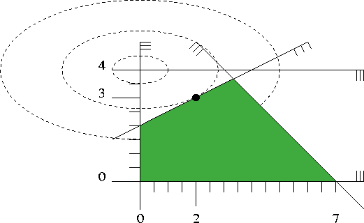
\[ \begin{array}{lrcl} \mbox{minimize} & x^2 + 4(y-4)^2 &(=& x^2 + 4y^2 - 32y + 64) \\ \mbox{subject to} & x + y &\leq& 7 \\ & -x + 2y &\leq& 4 \\ & x &\geq& 0 \\ & y &\geq& 0 \\ & y &\leq& 4 \end{array} \]
Figure 7.1 shows a picture. It depicts the five inequalities of the program, along with the feasible region (green), the set of points that satisfy all the five constraints. The dashed elliptic curves represent contour lines of the objective function, i.e., along each dashed curve, the objective function value is constant.
The global minimum of the objective function is attained at the point \( (0,4)\), and the minimum within the feasible region appears at the point \( (2,3)\) marked with a black dot. The value of the objective function at this optimal solution is \( 2^2 + 4(3-4)^2 = 8\).
Here is how this quadratic program can be solved in CGAL according to the first way (letting the model take care of the data). We use int as the input type, and MP_Float or Gmpz (which is faster and preferable if GMP is installed) as the exact type for the internal computations. In larger examples, it pays off to use double as input type in order to profit from the automatic floating-point filtering that takes place then.
For examples how to work with the input type double, we refer to Sections Working from Iterators and Customizing the Solver.
Note: For the quadratic objective function, the entries of the matrix \( 2D\) have to be provided, rather than \( D\). Although this is common to almost all quadratic programming solvers, it can easily be overlooked by a novice.
Asuming that GMP is installed, the output of the of the above program is:
status: OPTIMAL
objective value: 8/1
variable values:
0: 2/1
1: 3/1
If GMP is not installed, the values are of course the same, but numerator and denominator might have a common divisor that is not factored out.
Here, the program data must be available in MPSFormat (the MPSFormat page shows how our running example looks like in this format, and it briefly explains the format). Assuming that your working directory contains the file first_qp.mps, the following program will read and solve it, with the same output as before.
File QP_solver/first_qp_from_mps.cpp
The following program again solves our running example from above, with the same output, but this time with iterators over data stored in suitable containers. You can see that we also store zero entries here (in \( D\)). For this toy problem, the previous two approaches (program from data/stream) are clearly preferable, but Section Working from Iterators shows an example where it makes sense to use the iterator-based approach.
File QP_solver/first_qp_from_iterators.cpp
Note 1: The example shows an interesting feature of this approach: not all data need to come from containers. Here, the iterator over the vector of relations can be provided through the class Const_oneset_iterator<T>, since all entries of this vector are equal to SMALLER. The same could have been done with the vector fl for the finiteness of the lower bounds.
Note 2: The program type looks a bit scary, with its total of 9 template arguments, one for each iterator type. In Section Using Makers we show how the explicit construction of this type can be circumvented.
Let us reconsider the general form of (QP) from Section Which Programs can be Solved? above. If \( D=0\), the quadratic program is in fact a linear program, and in the case that the bound vectors \( l\) is the zero vector and all entries of \( u\) are \( \infty\), the program is said to be nonnegative. The package offers dedicated models and solution methods for these special cases.
From an interface perspective, this is just syntactic sugar: in the model Quadratic_program<NT>, we can easily set the default bounds so that a nonnegative program results, and a linear program is obtained by simply not inserting any \( D\)-entries. Even in the iterator-based approach (see QP_solver/first_qp_from_iterators.cpp), linear and nonnegative programs can easily be defined through suitable Const_oneset_iterator<T>-style iterators.
The main reason for having dedicated solution methods for linear and nonnegative programs is efficiency: if the solver knows that the program is linear, it can save some computations compared to the general solver that unknowingly has to fiddle around with a zero \( D\)-matrix. As in Section Robustness above, we can argue that checking in advance whether \( D=0\) is not an option in general, since this may require \( \Omega(n^2)\) time on the dense interface.
Similarly, if the solver knows that the program is nonnegative, it will be more efficient than under the general bounds \( \qpl\leq \qpx \leq \qpu\). You can argue that nonnegativity is something that could easily be checked in time \( O(n)\) beforehand, but then again nonnegative programs are so frequent that the syntactic sugar aspect becomes somewhat important. After all, we can save four iterators in specifying a nonnegative linear program in terms of the concept NonnegativeLinearProgram rather than LinearProgram.
Often, there are no bounds at all for the variables, i.e., all entries of \( \qpl\) are \( -\infty\), and all entries of \( \qpu\) are \( \infty\) (this is called a free program). There is no dedicated solution method for this case (a free quadratic or linear program is treated like a general quadratic or linear program), but all predefined models make it easy to specify all sorts of default bounds, covering the free case.
Let's go back to our first quadratic program from above and change it into a linear program by simply removing the quadratic part of the objective function:
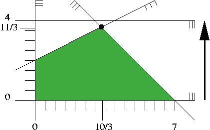
\[ \begin{array}{lrcl} \mbox{minimize} & - 32y + 64 \\ \mbox{subject to} & x + y &\leq& 7 \\ & -x + 2y &\leq& 4 \\ & x &\geq& 0 \\ & y &\geq& 0 \\ & y &\leq& 4 \end{array} \]
Figure 7.2 shows how this looks like. We will not visualize a linear objective function with contour lines but with arrows instead. The arrow represents the (direction) of the vector \( -c\), and we are looking for a feasible solution that is "extreme" in the direction of the arrow. In our small example, this is the unique point "on" the two constraints \( x_1+x_2\leq 7\) and \( -x_1+x_2\leq 4\), the point \( (10/3,11/3)\) marked with a black dot. The optimal objective function value is \( -32(11/3)+64=-160/3\).
Here is CGAL code for solving it, using the dedicated LP solver, and according to the three ways for constructing a program that we have already discussed in Section How to Enter and Solve a Program.
QP_solver/first_lp_from_mps.cpp
QP_solver/first_lp_from_iterators.cpp
In all cases, the output is
status: OPTIMAL
objective value: -160/3
variable values:
0: 10/3
1: 11/3
If we go back to our first quadratic program and remove the constraint \( y\leq 4\), we arrive at a nonnegative quadratic program:
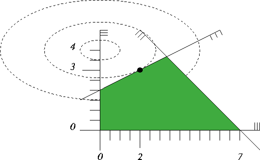
\[ \begin{array}{lrcl} \mbox{minimize} & x^2 + 4(y-4)^2 &(=& x^2 + 4y^2 - 32y + 64) \\ \mbox{subject to} & x + y &\leq& 7 \\ & -x + 2y &\leq& 4 \\ & x,y &\geq& 0 \end{array} \]
Figure 7.3 contains the illustration; since the constraint \( y\leq 4\) was redundant, the feasible region and the optimal solution do not change.
The following programs (using the dedicated solver for nonnegative quadratic programs) will therefore again output
status: OPTIMAL
objective value: 8/1
variable values:
0: 2/1
1: 3/1
QP_solver/first_nonnegative_qp.cpp
QP_solver/first_nonnegative_qp_from_mps.cpp
QP_solver/first_nonnegative_qp_from_iterators.cpp
Finally, a dedicated model and function is available for nonnnegative linear programs as well. Let's take our linear program from above and remove the constraint \( y\leq 4\) to obtain a nonnegative linear program. At the same time we remove the constant objective function term to get a "minimal" input and a "shortest" program; the optimal value is \( -32(11/3)=-352/3\).
\[ \begin{array}{lrcl} \mbox{minimize} & - 32y \\ \mbox{subject to} & x + y &\leq& 7 \\ & -x + 2y &\leq& 4 \\ & x,y &\geq& 0 \\ \end{array} \]
This can be solved by any of the following three programs
QP_solver/first_nonnegative_lp.cpp
QP_solver/first_nonnegative_lp_from_mps.cpp
QP_solver/first_nonnegative_lp_from_iterators.cpp
The output will always be
status: OPTIMAL
objective value: -352/3
variable values:
0: 10/3
1: 11/3
Here we present a somewhat more advanced example that emphasizes the usefulness of solving linear and quadratic programs from iterators. Let's look at a situation in which a linear program is given implicitly, and access to it is gained through properly constructed iterators.
The problem we are going to solve is the following: given points \( p_1,\ldots p_{n}\) in \( d\)-dimensional space and another point \( p\): is \( p\) in the convex hull of \( \{p_1,\ldots,p_{n}\}\)? In formulas, this is the case if and only if there are real coefficients \( \lambda_1,\ldots,\lambda_n\) such that \( p\) is a convex combination of \( p_1,\ldots,p_n\): \( p = \ccSum{j=1}{n}{~\lambda_j~p_j}, \quad \ccSum{j=1}{n}{~\lambda_j} = 1, \quad \lambda_j \geq 0 \mbox{~for all $j$.} \)
The problem of testing the existence of such \( \lambda_j\) can be expressed as a linear program. It becomes particularly easy when we use the homogeneous representations of the points: if \( q_1,\ldots,q_n,q\in\mathbb{R}^{d+1}\) are homogeneous coordinates for \( p_1,\ldots,p_n,p\) with positive homogenizing coordinates \( h_1,\ldots,h_n,h\), we have
\[$q_j = h_j \cdot (p_j \mid 1) \mbox{~for all $j$, and~} q = h \cdot (p\mid 1).\]
Now, nonnegative \(\lambda_1,\ldots,\lambda_n\) are suitable coefficients for a convex combination if and only if
\[\ccSum{j=1}{n}{~ \lambda_j(p_j \mid 1)} = (p\mid 1), \]
equivalently, if there are \(\mu_1,\ldots,\mu_n\) (with \(\mu_j = \lambda_j \cdot h/{h_j}\) for all \(j\)) such that
\[\ccSum{j=1}{n}{~\mu_j~q_j} = q, \quad \mu_j \geq 0\mbox{~for all $j$}.\]
The linear program now tests for the existence of nonnegative \( \mu_j\) that satisfy the latter equation. Below is the code; it defines a function that solves the linear program, given \( p\) and \( p_1,\ldots,p_n\) (through an iterator range). The only (mild) trickery involved is the construction of the nested iterator through a fixed column of the constraint matrix \( A\). We get this from transforming the iterator through the points using a functor that maps a point to an iterator through its homogeneous coordinates.
File QP_solver/solve_convex_hull_containment_lp.h
To see this in action, let us call it with \( p_1=(0,0), p_2=(10,0), p_3=(0,10)\) fixed (they define a triangle) and all integral points \( p\) in \( [0,10]^2\). We know that \( p\) is in the convex hull of \( \{p_1,p_2,p_3\}\) if and only if its two coordinates sum up to \( 10\) at most. As the exact type, we use MP_Float or Gmpzf (which is faster and preferable if GMP is installed).
File QP_solver/convex_hull_containment.cpp
You already noticed in the previous example that the actual template arguments for Nonnegative_linear_program_from_iterators<A_it, B_it, R_it, C_it> can be quite elaborate, and this only gets worse if you plug more iterators into each other. In general, you want to construct a program from given expressions for the iterators, but the types of these expressions are probably very complicated and difficult to look up.
You can avoid the explicit construction of the type Nonnegative_linear_program_from_iterators<A_it, B_it, R_it, C_it> if you only need an expression of it, e.g. to pass it directly as an argument to the solving function. Here is an alternative version of QP_solver/solve_convex_hull_containment_lp.h that shows how this works. In effect, you get shorter and more readable code.
File QP_solver/solve_convex_hull_containment_lp2.h
If you have a solution \( \qpx^*\) of a linear or quadratic program, the "important" variables are typically the ones that are not on their bounds. In case of a nonnegative program, these are the nonzero variables. Going back to the example of the previous Section Working from Iterators, we can easily interpret their importance: the nonzero variables correspond to points \( p_j\) that actually contribute to the convex combination that yields \( p\).
The following example shows how we can access the important variables, using the iterators basic_variable_indices_begin() and basic_variable_indices_end().
We generate a set of points that form a 4-gon in \( [0,4]^2\), and then find the ones that contribute to the convex combinations of all 25 lattice points in \( [0,4]^2\). If the lattice point in question is not in the 4-gon, we simply output this fact.
File QP_solver/important_variables.cpp
It turns out that exactly three of the four points contribute to any convex combination, even through there are lattice points that lie in the convex hull of less than three of the points. This shows that the set of basic variables that we access in the example does not necessarily coincide with the set of important variables as defined above. In fact, it is only guaranteed that a non-basic variable attains one of its bounds, but there might be basic variables that also have this property. In linear and quadratic programming terms, such a situation is called a degeneracy.
There is also the concept of an important constraint: this is typically a constraint in the system \( A\qpx\qprel\qpb\) that is satisfied with equality at \( \qpx^*\). Program QP_solver/first_qp_basic_constraints.cpp shows how these can be accessed, using the iterators basic_constraint_indices_begin() and basic_constraint_indices_end().
Again, we have a disagreement between "basic" and "important": it is guaranteed that all basic constraints are satisfied with equality at \( \qpx^*\), but there might be non-basic constraints that are satisfied with equality as well.
Suppose the solver tells you that the problem you have entered is infeasible. Why should you believe this? Similarly, you can quite easily verify that a claimed optimal solution is feasible, but why is there no better one?
Certificates are proofs that the solver can give you in order to convince you that what it claims is indeed true. The archetype of such a proof is Farkas Lemma [1].
Farkas Lemma: Either the inequality system
\[ \begin{array}{rcl} A \qpx & \leq & \qpb \\ \qpx & \geq & 0 \end{array} \]
has a solution \( \qpx^*\), or there exists a vector \( \qpy\) such that
\[ \begin{array}{rcl} \qpy &\geq& 0\\ \qpy^TA &\geq& 0\\ \qpy^T\qpb & < & 0, \end{array} \]
but not both.
Thus, if someone wants to convince you that the first system in the Farkas Lemma is infeasible, that person can simply give you a vector \( \qpy\) that solves the second system. Since you can easily verify yourself that the \( \qpy\) you got satisfies this second system, you now have a certificate for the infeasibility of the first system, assuming that you believe in Farkas Lemma.
Here we show how the solver can convince you. We first set up an infeasible linear program with constraints of the type \( A\qpx\leq \qpb, \qpx\geq 0\); then we solve it and ask for a certificate. Finally, we verify the certificate by simply checking the inequalities of the second system in Farkas Lemma.
File QP_solver/infeasibility_certificate.cpp
There are similar certificates for optimality and unboundedness that you can see in action in the programs QP_solver/optimality_certificate.cpp and QP_solver/unboundedness_certificate.cpp. The underlying variants of Farkas Lemma are somewhat more complicated, due to the mixed relations in \( \qprel\) and the general bounds. The certificate section of Quadratic_program_solution<ET> gives the full picture and mathematically proves the correctness of the certificates.
Sometimes it is necessary to alter the default behavior of the solver. This can be done by passing a suitably prepared object of the class Quadratic_program_options to the solution functions. Most options concern "soft" issues like verbosity, but there are two notable case where it is of critical importance to be able to change the defaults.
The filtered version of the solver that is used for some problems by default on input type double internally constructs double-approximations of exact multiprecision values. If these exact values are extremely large, this may lead to infinite double values and incorrect results. In debug mode, the solver will notice this through a certificate cross-check in the end (or even earlier). In this case, it is advisable to explicitly switch to a non-filtered pricing strategy, see Quadratic_program_pricing_strategy.
Hint: If you have a program where the number of variables \( n\) and the number of constraints \( m\) have the same order of magnitude, the filtering will usually have no dramatic effect on the performance, so in that case you might as well switch to QP_PARTIAL_DANTZIG to be safe from the issue described here (see QP_solver/cycling.cpp for an example that shows how to change the pricing strategy).
Consider the following program. It reads a nonnegative linear program from the file cycling.mps (which is in the example directory as well), and then solves it in verbose mode, using Bland's rule, see Quadratic_program_pricing_strategy.
File QP_solver/cycling.cpp
If you comment the line
options.set_pricing_strategy(CGAL::QP_BLAND); // Bland's rule
you will see that the solver cycles: the verbose mode outputs the same sequence of six iterations over and over again. By switching to QP_BLAND, the solution process typically slows down a bit (it may also speed up in some cases), but now it is guaranteed that no cycling occurs.
In general, the verbose mode can be of use when you are not sure whether the solver "has died", or whether it simply takes very long to solve your problem. We refer to the class Quadratic_program_options for further details.
Here we want to show what you can expect from the solver's performance in a specific application; we don't know whether this application is typical in your case, and we make no claims whatsoever about the performance in other applications.
Still, the example shows that the performance can be dramatically affected by switching between pricing strategies, and we give some hints on how to achieve good performance in general.
The application is the one already discussed in Section Working from Iterators above: testing whether a point is in the convex hull of other points. To be able to switch between pricing strategies, we add another parameter of type Quadratic_program_options to the function solve_convex_hull_containment_lp that we pass on to the solution function:
File QP_solver/solve_convex_hull_containment_lp3.h
Now let us test containment of the origin in the convex hull of \( n\) random points in \( [0,1]^d\) (it will most likely not be contained, and it turns out that this is the most expensive case). In the program below, we use \( d=10\) and \( n=100,000\), and we comment on some other combinations of \( n\) and \( d\) below (feel free to experiment with still other values).
File QP_solver/convex_hull_containment_benchmarks.cpp
If you compile with the macros NDEBUG or CGAL_QP_NO_ASSERTIONS set (this is essential for good performance!!), you will see runtimes that qualitatively look as follows (on your machine, the actual runtimes will roughly be some fixed multiples of the numbers in the table below, and they might vary with the random choices). The default choice of the pricing strategy in that case is QP_PARTIAL_FILTERED_DANTZIG.
| Strategy | Runtime in seconds |
|---|---|
QP_CHOOSE_DEFAULT | 0.32 |
QP_DANTZIG | 10.7 |
QP_PARTIAL_DANTZIG | 3.72 |
QP_BLAND | 3.65 |
QP_FILTERED_DANTZIG | 0.43 |
QP_PARTIAL_FILTERED_DANTZIG | 0.32 |
We clearly see the effect of filtering: we gain a factor of ten, roughly, compared to the next best non-filtered variant.
The filtering effect is amplified if the points/dimension ratio becomes larger. This is what you might see in dimension three, with one million points.
| Strategy | Runtime in seconds |
|---|---|
QP_CHOOSE_DEFAULT | 1.34 |
QP_DANTZIG | 47.6 |
QP_PARTIAL_DANTZIG | 15.6 |
QP_BLAND | 16.02 |
QP_FILTERED_DANTZIG | 1.89 |
QP_PARTIAL_FILTERED_DANTZIG | 1.34 |
In general, if your problem has a high variable/constraint or constraint/variable ratio, then filtering will typically pay off. In such cases, it might be beneficial to encode your problem using input type double in order to profit from the filtering (but see the issue discussed in Section Exponent Overflow in Double Using Floating-Point Filters).
Conversely, the filtering effect deteriorates if the points/dimension ratio becomes smaller.
| Strategy | Runtime in seconds |
|---|---|
QP_CHOOSE_DEFAULT | 3.05 |
QP_DANTZIG | 78.4 |
QP_PARTIAL_DANTZIG | 45.9 |
QP_BLAND | 33.2 |
QP_FILTERED_DANTZIG | 3.36 |
QP_PARTIAL_FILTERED_DANTZIG | 3.06 |
If the points/dimension ratio tends to a constant, filtering is no longer a clear winner. The reason is that in this case, the necessary exact calculations with multiprecision numbers dominate the overall runtime.
| Strategy | Runtime in seconds |
|---|---|
QP_CHOOSE_DEFAULT | 2.65 |
QP_DANTZIG | 5.55 |
QP_PARTIAL_DANTZIG | 5.6 |
QP_BLAND | 4.46 |
QP_FILTERED_DANTZIG | 2.65 |
QP_PARTIAL_FILTERED_DANTZIG | 2.61 |
In general, if you have a program where the number of variables and the number of constraints have the same order of magnitude, then the saving gained from using the filtered approach is typically small. In such a situation, you should consider switching to a non-filtered variant in order to avoid the rare issue discussed in Section Exponent Overflow in Double Using Floating-Point Filters altogether.
 1.8.4
1.8.4