

|
CGAL 4.8 - 2D Visibility
|
|
CGAL 4.8 - 2D Visibility
|
This package provides functionality to compute the visibility region within polygons in two dimensions. The package is based on the package 2D Arrangements and uses CGAL::Arrangement_2 as the fundamental class to specify the input as well as the output. Hence, a polygon \( P \) is represented by a bounded arrangement face \( f \) that does not have any isolated vertices and any edge that is adjacent to \( f \) separates \( f \) from another face. Note that \( f \) may contain holes. Similarly, a simple polygon is represented by a face without holes.
Given two points \( p \) and \( q \) in \( P \), they are said to be visible to each other iff the segment \( pq \subset P \), where \( P \) is considered to be closed, that is, \(\partial P \subset P\). For a query point \( q \in P \), the set of points that are visible from \( q \) is defined as the visibility region of \( q \), denoted by \( V_q \)
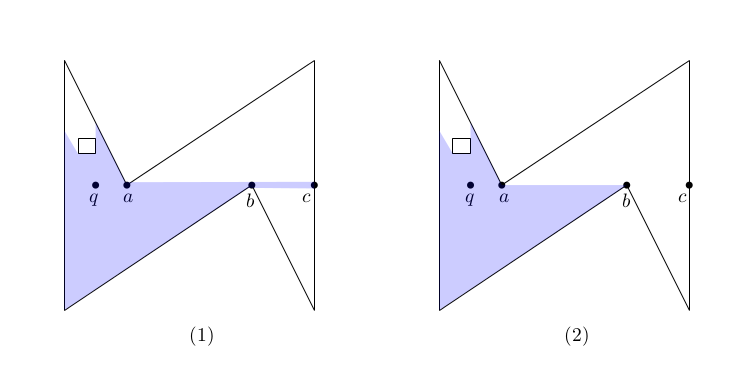
As illustrated in Figure 23.1 (1) the visibility region \( V_q \) of a query point \( q \) may not be a polygon. In the figure, all labeled points are collinear, which implies that the point \( c \) is visible to \( q \), that is, the segment \( bc \) is part of \( V_q \). We call such low dimensional features that are caused by degeneracies needles. However, for many applications these needles are actually irrelevant. Moreover, for some algorithms it is even more efficient to ignore needles in the first place. Therefore, this package offers also functionality to compute the regularized visibility area \( \overline{V_q} = closure(interior(V_q)) = (V_q\setminus\partial V_q) \cup \partial (V_q\setminus\partial V_q)\), as shown in Figure 23.1 (2). For more information about regularization, refer to Chapter 2D Regularized Boolean Set-Operations.
Answering visibility queries is, in many ways, similar to answering point-location queries. Thus, we use the same design used to implement 2D Arrangements point location. Each of the various visibility class templates employs a different algorithm or strategy for answering queriesThe term strategy is borrowed from the design-pattern taxonomy [3]. A strategy provides the means to define a family of algorithms, each implemented by a separate class. All classes that implement the various algorithms are made interchangeable, letting the algorithm in use vary according to the user choice.. Similar to the point-location case, some of the strategies require preprocessing. Thus, before a visibility object is used to answer visibility queries, it must be attached to an arrangement object. Afterwards, the visibility object observes changes to the attached arrangement. Hence, it is possible to modify the arrangement after attaching the visibility object. However, this feature should be used with caution as each change to the arrangement also requires an update of the auxiliary data structures in the attached object.
An actual query is performed by giving the view point \( p \) and its containing face \( f \) (which must represent a valid polygon) to a visibility object. For more details see the documentation of the overloaded member function Visibility_2::compute_visibility().
The following models of the Visibility_2 concept are provided:
| Class | Function | Preprocessing | Query | Algorithm |
|---|---|---|---|---|
Simple_polygon_visibility_2 | simple polygons | No | \( O(n) \) time and \( O(n) \) space | B. Joe and R. B. Simpson[4] |
Rotational_sweep_visibility_2 | polygons with holes | No | \( O(n\log n) \) time and \( O(n) \) space | T. Asano[1] |
Triangular_expansion_visibility_2 | polygons with holes | \( O(n) \) time and \( O(n) \) space | \( O(nh) \) time and \( O(n) \) space. | Bungiu et al.[2] |
Where \( n \) denotes the number of vertices of \( f \) and \( h \) the number of holes+1.
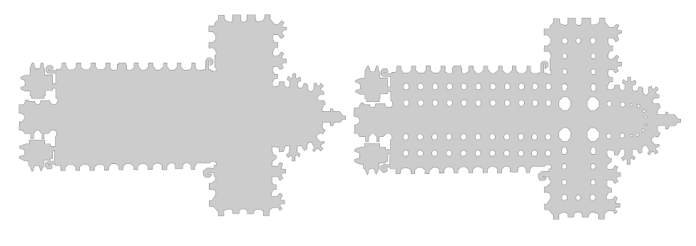
The left hand side of Figure Figure 23.2 depicts the outer boundary of a cathedral, which is a simple polygon with 565 vertices. The right hand side shows the cathedral also with its inner pillars, which is a polygon (with holes) with 1153 vertices. The following table shows the total running time consumption of the computation of all visibility polygons for all vertices of the cathedral.
| Boundary Cathedral | total preprocessing time | total query time |
|---|---|---|
Simple_polygon_visibility_2 | - | 0.38 |
Rotational_sweep_visibility_2 | - | 1.01 |
Triangular_expansion_visibility_2 | 0.01 | 0.06 |
The second table shows the same for the complete cathedral. The table does not report the time for Simple_polygon_visibility_2 as this algorithm can only handle simple polygons.
| Complete Cathedral | total preprocessing time | total query time |
|---|---|---|
Rotational_sweep_visibility_2 | - | 1.91 |
Triangular_expansion_visibility_2 | 0.01 | 0.04 |
Thus, in general we recommend to use Triangular_expansion_visibility_2 even if the polygon is simple. The main advantage of the algorithm is its locality. After the triangle that contains the query point is located in the triangulation, the algorithm explores neighboring triangles, but only those that are actually seen. In this sense the algorithm can be considered as output sensitive. Note that the Triangular_expansion_visibility_2 algorithm performs better on the full cathedral since the additional pillars block the view early in many cases. However, if the simple polygon is rather convex (i.e., nearly all boundary is seen) or if only one (or very little) queries are required, using one of the algorithms that does not require preprocessing is advantageous.
The following example shows how to obtain the regularized and non-regularized visibility regions.
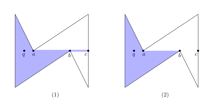
The visibility region of \( q \) in a simple polygon: (1) non-regularized visibility; and (2) regularized visibility.
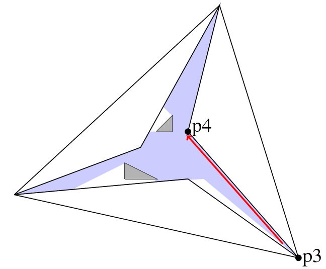
The following example shows how to obtain the regularized visibility region using the model Triangular_expansion_visibility_2, see Figure 23.4. The arrangement has six bounded faces and an unbounded face. The query point \( q \) is on a vertex. The red arrow denotes the halfedge \( \overrightarrow{pq} \), which also identifies the face in which the visibility region is computed.
This package was first developed during Google Summer of Code 2013: Francisc Bungiu developed the CGAL::Simple_polygon_visibility_2, Kan Huang developed the CGAL::Rotational_sweep_visibility_2, and Michael Hemmer developed the CGAL::Triangular_expansion_visibility_2.
During Google Summer of Code 2014 Ning Xu fixed a bug in CGAL::Simple_polygon_visibility_2 and improved the testsuite.
 1.8.4
1.8.4