|
CGAL 4.9 - Point Set Processing
|
|
CGAL 4.9 - Point Set Processing
|
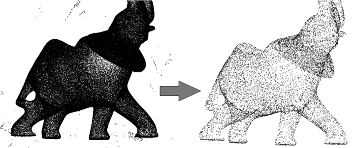
This CGAL component implements methods to analyze and process 3D point sets. The input is an unorganized 3D point set, possibly with normal attributes (unoriented or oriented). The input point set can be analyzed to measure geometric properties such as average spacing between the points and their k nearest neighbors. It can be processed with functions devoted to the simplification, regularization, upsampling, outlier removal, smoothing, normal estimation and normal orientation. The processing of point sets is often needed in applications dealing with measurement data, such as surface reconstruction from laser scanned data (see Figure 68.1).
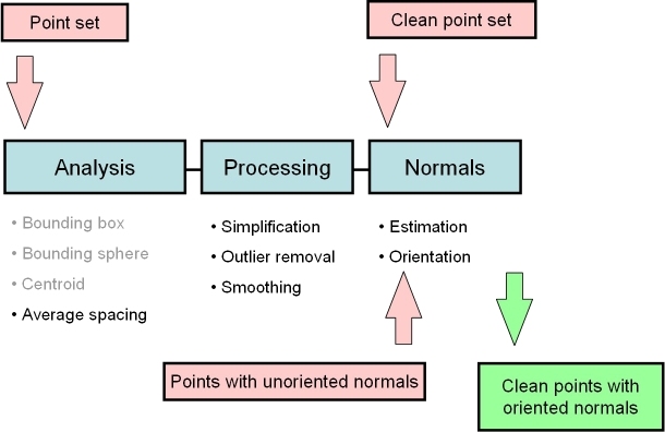
In the context of surface reconstruction we can position the elements of this component along the common surface reconstruction pipeline (Figure 68.2) which involves the following steps:
The algorithms of this component take as input parameters iterator ranges of 3D points, or of 3D points with normals. The property maps are used to access the point or normal information from the input data, so as to let the user decide upon the implementation of a point with normal. The latter can be represented as, e.g., a class derived from the CGAL 3D point, or as a std::pair<Point_3<K>, Vector_3<K>>, or as a boost::tuple<..,Point_3<K>, ..., Vector_3<K> >.
The following classes described in Chapter CGAL and Boost Property Maps provide property maps for the implementations of points with normals listed above:
Identity_property_map<T>First_of_pair_property_map<Pair> and Second_of_pair_property_map<Pair>Nth_of_tuple_property_map<N, Tuple>Identity_property_map<Point_3> is the default value of the position property map expected by all functions in this component.
See below examples using pair and tuple property maps.
Users of this package may use other types to represent positions and normals if they implement the corresponding property maps.
Points and normals can even be stored in separate containers and accessed by their index, as any built-in vector is also a property map.
File Point_set_processing_3/grid_simplify_indices.cpp
We provide functions to read and write sets of points or sets of points with normals from the following ASCII file formats: XYZ (three point coordinates x y z per line or three point coordinates and three normal vector coordinates x y z nx ny nz per line), OFF (Object File Format) [6] and PLY (Polygon File Format).
read_xyz_points() and read_xyz_points_and_normals()read_off_points() and read_off_points_and_normals()read_ply_points(), read_ply_points_and_normals() and read_ply_custom_points()write_xyz_points() and write_xyz_points_and_normals()write_off_points() and write_off_points_and_normals()write_ply_points() and write_ply_points_and_normals()Note that PLY reading functions accepts binary PLY format in addition of ASCII. read_ply_custom_points() provides the user with a means to read any point property from a PLY file (for example, colors), see Example of custom PLY reader.
The following example reads a point set from an input file and writes it to a file, both in the XYZ format. Positions and normals are stored in pairs and accessed through property maps.
File Point_set_processing_3/read_write_xyz_point_set_example.cpp
PLY files are designed to embed an arbitrary number of additional attributes. More specifically, point sets may contain normal vectors, visibility vectors, RGB colors, intensity, etc. As it is not possible to provide dedicated functions to every possible combination of PLY properties, CGAL provides a simple way to write custom PLY readers so that the user can adapt its programs to its PLY input.
The function read_ply_custom_points() uses the concept PlyInterpreter to read specific properties defined by the user. CGAL provides, for this concept, the model CGAL::Ply_interpreter_points_and_normals_3: it is the standard interpreter that is used internally by read_ply_points() and read_ply_points_and_normals().
The following example shows how to define a custom interpreter that reads a point set with points, normals and RGB colors, and stores these attributes in user-defined containers.
File Point_set_processing_3/read_ply_points_with_colors_example.cpp
Function compute_average_spacing() computes the average spacing of all input points to their k nearest neighbor points, k being specified by the user. As it provides an order of a point set density, this function is used downstream the surface reconstruction pipeline to automatically determine some parameters such as output mesh sizing for surface reconstruction.
The following example reads a point set in the xyz format and computes the average spacing. Index, position and color are stored in a tuple and accessed through property maps.
File Point_set_processing_3/average_spacing_example.cpp
Note that other functions such as centroid or bounding volumes are found in other CGAL components:
Function remove_outliers() deletes a user-specified fraction of outliers from an input point set. More specifically, it sorts the input points in increasing order of average squared distances to their k nearest neighbors and deletes the points with largest value.
The following example reads a point set and removes 5% of the points. It uses the Identity_property_map<Point_3> property map (optional as it is the default position property map of all functions in this component.)
File Point_set_processing_3/remove_outliers_example.cpp
Four simplification functions are devised to reduce an input point set.
Function random_simplify_point_set() randomly deletes a user-specified fraction of points from the input point set. This algorithm is fast.
Function grid_simplify_point_set() considers a regular grid covering the bounding box of the input point set, and clusters all points sharing the same cell of the grid by picking as representant one arbitrarily chosen point. This algorithm is slower than random_simplify_point_set().
Function hierarchy_simplify_point_set() provides an adaptive simplification of the point set through local clusters [5]. The size of the clusters is either directly selected by the user or it automatically adapts to the local variation of the point set.
Function wlop_simplify_and_regularize_point_set() not only simplifies, but also regularizes downsampled points. This is an implementation of the Weighted Locally Optimal Projection (WLOP) algorithm [2].
The following example reads a point set and simplifies it by clustering.
File Point_set_processing_3/grid_simplification_example.cpp
The following example reads a point set and produces a set of clusters.
File Point_set_processing_3/hierarchy_simplification_example.cpp
The hierarchy simplification algorithm recursively split the point set in two until each cluster's size is less than the parameter size.

size parameter: \(10\), \(100\) and \(1000\). In the 3 cases, var_max \(=1/3\). In addition to the size parameter, a variation parameter allows to increase simplification in monotoneous regions. For each cluster, a surface variation measure is computed using the sorted eigenvalues of the covariance matrix:
\[ \sigma(p) = \frac{\lambda_0}{\lambda_0 + \lambda_1 + \lambda_2}. \]
This function goes from \(0\) if the cluster is coplanar to \(1/3\) if it is fully isotropic. If a cluster's variation is above var_max, it is split. If var_max is equal to \(1/3\), this parameter has no effect and the clustering is regular on the whole point set.

var_max parameter: \(0.00001\), \(0.001\) and \(0.1\). In the 3 cases, size \(=1000\). The following example reads a point set, simplifies and regularizes it by WLOP.
File Point_set_processing_3/wlop_simplify_and_regularize_point_set_example.cpp

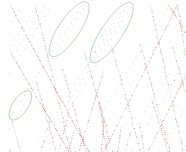
Computing density weights for each point is an optional preprocessing. For example, as shown in the following figure, when require_uniform_sampling is set to false, WLOP preserves the intrinsic non-uniform sampling of the original points; if require_uniform_sampling is set to true, WLOP is resilient to non-uniform sampling and generates sample points with more uniform distribution, at the expense of computational time.

require_uniform_sampling = false. Right: require_uniform_sampling=true. Usually, the neighborhood of sample points should include at least two rings of neighboring sample points. Using a small neighborhood size may not be able to generate regularized result, while using big neighborhood size will make the sample points shrink into the interior of the local surface (under-fitting). The function will use a neighborhood size estimation if this parameter value is set to default or smaller that zero.

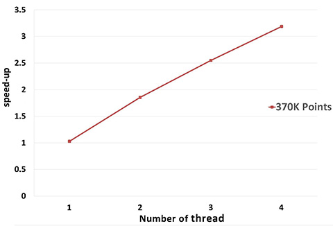
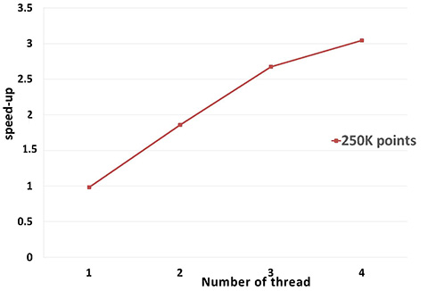
A parallel version of WLOP is provided and requires the executable to be linked against the Intel TBB library. To control the number of threads used, the user may use the tbb::task_scheduler_init class. See the TBB documentation for more details. We provide below a speed-up chart generated using the parallel version of the WLOP algorithm. The machine used is a PC running Windows 7 64-bits with a 4-core i7-4700HQ@2.40GHz CPU with 8GB of RAM.
Two smoothing functions are devised to smooth an input point set.
Function jet_smooth_point_set() smooths the input point set by projecting each point onto a smooth parametric surface patch (so-called jet surface) fitted over its k nearest neighbors.
Function bilateral_smooth_point_set() smooths the input point set by iteratively projecting each point onto the implicit surface patch fitted over its k nearest neighbors. Bilateral projection preserves sharp features according to the normal (gradient) information. Normals are thus required as input. For more details, see section 4 of [3].
The following example generates a set of 9 points close to the xy plane and smooths them using 8 nearest neighbors:
File Point_set_processing_3/jet_smoothing_example.cpp
The following example reads a set of points with normals and smooths them via bilateral smoothing:
File Point_set_processing_3/bilateral_smooth_point_set_example.cpp

Performance: A parallel version of bilateral smoothing is provided and requires the executable to be linked against the Intel TBB library. The number of threads used is controlled through the tbb::task_scheduler_init class. See the TBB documentation for more details. We provide below a speed-up chart generated using the parallel version of the bilateral smoothing algorithm. The machine used is a PC running Windows 7 64-bits with a 4-core i7-4700HQ@2.40GHz CPU with 8GB of RAM.
Assuming a point set sampled over an inferred surface S, two functions provide an estimate of the normal to S at each point. The result is an unoriented normal vector for each input point.
Function jet_estimate_normals() estimates the normal direction at each point from the input set by fitting a jet surface over its k nearest neighbors. The default jet is a quadric surface. This algorithm is well suited to point sets scattered over curved surfaces.
Function pca_estimate_normals() estimates the normal direction at each point from the set by linear least squares fitting of a plane over its k nearest neighbors. This algorithm is simpler and faster than jet_estimate_normals().
Function vcm_estimate_normals() estimates the normal direction at each point from the set by using the Voronoi Covariance Measure of the point set. This algorithm is more complex and slower than the previous algorithms. It is based on the article [4].
Function mst_orient_normals() orients the normals of a set of points with unoriented normals using the method described by Hoppe et al. in Surface reconstruction from unorganized points [1]. More specifically, this method constructs a Riemannian graph over the input points (the graph of the k nearest neighbor points) and propagates a seed normal orientation within a minimum spanning tree computed over this graph. The result is an oriented normal vector for each input unoriented normal, except for the normals which cannot be successfully oriented.
The following example reads a point set from a file, estimates the normals through PCA over the 6 nearest neighbors and orients the normals:
File Point_set_processing_3/normals_example.cpp
The function edge_aware_upsample_point_set() generates a denser point set from an input point set. This has applications in point-based rendering, hole filling, and sparse surface reconstruction. The algorithm can progressively upsample the point set while approaching the edge singularities. See [3] for more details.
The following example reads a point set from a file, upsamples it to get a denser result.
File Point_set_processing_3/edge_aware_upsample_point_set_example.cpp
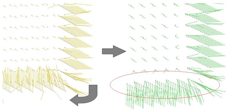
This parameter controls where the new points are inserted. Larger values of edge-sensitivity give higher priority to inserting points along the sharp features. For example, as shown in the following figure, high value is preferable when one wants to insert more points on sharp features, where the local gradient is high, e.g., darts, cusps, creases and corners. In contrast, points are evenly inserted when edge_sensitivity is set to 0. The range of possible value is [0, 1].

This parameter controls the preservation of sharp features.

Usually, the neighborhood of sample points should include at least one ring of neighboring sample points. Using small neighborhood size may not be able to insert new points. Using big neighborhood size can fill small holes, but points inserted on the edges could be irregular. The function will use a neigbhorhood size estimation if this parameter value is set to default or smaller than zero.

Function vcm_is_on_feature_edge() indicates if a points belong to a feature edges of the point set using its Voronoi Covariance Measure. It is based on the article [4].
It first computes the VCM of the points set using compute_vcm(). Then, it estimates which points belong to a sharp edge by testing if a ratio of eigenvalues is greater than a given threshold.
The following example reads a point set from a file, estimates the points that are on sharp edges:
File Point_set_processing_3/edges_example.cpp
Pierre Alliez and Laurent Saboret contributed the initial component. Nader Salman contributed the grid simplification. Started from GSoC'2013, three new algorithms were implemented by Shihao Wu and Clément Jamin: WLOP, bilateral smoothing and upsampling. Started from GSoC'2014, Jocelyn Meyron with the help of Quentin Mérigot introduced the computation of the Voronoi covarience measure of a point set, as well as the normal and feature edge estimation functions based on it.