

|
CGAL 5.0.2 - Approximation of Ridges and Umbilics on Triangulated Surface Meshes
|
|
CGAL 5.0.2 - Approximation of Ridges and Umbilics on Triangulated Surface Meshes
|
This chapter describes the CGAL package for the approximating the ridges and umbilics of a smooth surface discretized by a triangle mesh. Given a smooth surface, a ridge is a curve along which one of the principal curvatures has an extremum along its curvature line. An umbilic is a point at which both principal curvatures are equal. Ridges define a singular curve, i.e., a self-intersecting curve, and umbilics are special points on this curve. Ridges are curves of extremal curvature and therefore encode important informations used in segmentation, registration, matching and surface analysis. Based on the results of the article [2], we propose algorithms to identify and extract different parts of this singular ridge curve as well as umbilics on a surface given as a triangulated surface mesh. Differential quantities associated to the mesh vertices are assumed to be given for these algorithms; such quantities may be computed by the package Estimation of Local Differential Properties of Point-Sampled Surfaces.
Note that this package needs the third party library Eigen for linear algebra operations.
Section Ridges and Umbilics of a Smooth Surface presents the basics of the theory of ridges and umbilics on smooth surfaces. Sections Approximating Ridges on Triangulated Surface Meshes and Approximating Umbilics on Triangulated Surface Meshes present algorithms for approximating the ridges and umbilics (of a smooth surface) from a triangle mesh. Section Software Design gives the package specifications, while example calls to functions of the package are provided in Section Examples.
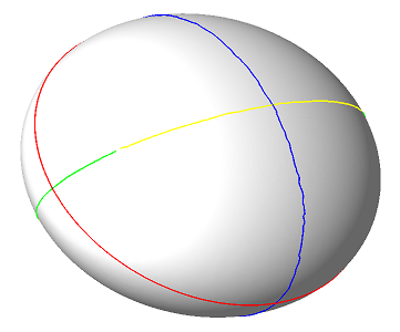
For a detailed introduction to ridges and related topics, the reader may consult [3],cgal:p-gd-01, as well as the following survey article [1]. In the sequel, we just introduce the basic notions so as to explain our algorithms. Consider a smooth embedded surface, and denote \( k_1\) and \( k_2\) the principal curvatures, with \( k_1\geq k_2\). Umbilics are the points where \( k_1=k_2\). For any non umbilical point, the corresponding principal directions of curvature are well defined, and we denote them \( d_1\) and \( d_2\). In local coordinates, we denote \( \langle , \rangle\) the inner product induced by the ambient Euclidean space, and \( dk_1\), \( dk_2\) the gradients of the principal curvatures. Ridges, illustrated in Figure 73.2 for the standard ellipsoid, are defined by:
Definition.A non umbilical point is called
a max ridge point, if the extremality coefficient \( b_0=\langle dk_1,d_1 \rangle\) vanishes, i.e. \( b_0=0\).
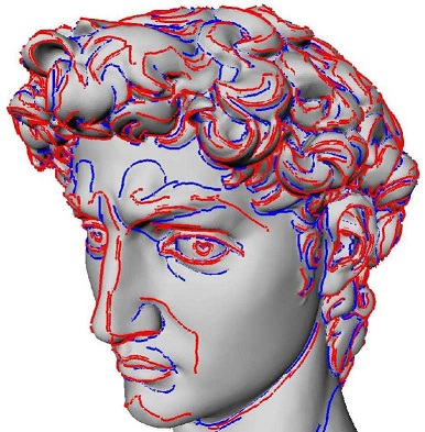
The previous characterization of ridges involves third-order differential properties. Using fourth-order differential quantities, a ridge point can further be qualified as elliptic if it corresponds to a maximum of \( k_1\) or a minimum of \( k_2\), or hyperbolic otherwise. Hence we end up with four types of ridges, namely: MAX_ELLIPTIC_RIDGE, MAX_HYPERBOLIC_RIDGE, MIN_ELLIPTIC_RIDGE, MIN_HYPERBOLIC_RIDGE, which are illustrated in Figure 73.2. Also of interest are the crest lines, a crest line being an elliptic ridge which is a maximum of \( \max(|k_1|,|k_2|)\). Crest lines form a subset of elliptic ridges, and can be seen as the visually most salient curves on a surface. Hence we provide the two additional ridge types MAX_CREST_RIDGE and MIN_CREST_RIDGE, which are illustrated in Figure 73.1.
At any point of the surface which is not an umbilic, principal directions \( d_1, d_2\) are well defined, and these (non oriented) directions together with the normal vector \( n\) define two direct orthonormal frames. If \( v_1\) is a unit vector of direction \( d_1\) then there exists a unique unit vector \( v_2\) so that \( (v_1,v_2,n)\) is direct, that is has the same orientation as the canonical basis of the ambient \( 3d\) space (and the other possible frame is \( (-v_1,-v_2,n)\)). In the coordinate systems \( (v_1,v_2,n)\), the surface has the following canonical form, known as the Monge form :
\begin{eqnarray} z(x,y) = & \frac{1}{2}(k_1x^2 + k_2y^2)+ \frac{1}{6}(b_0x^3+3b_1x^2y+3b_2xy^2+b_3y^3) \\ & +\frac{1}{24}(c_0x^4+4c_1x^3y+6c_2x^2y^2+4c_3xy^3+c_4y^4) + h.o.t \end{eqnarray}
The Taylor expansion of \( k_1\) (resp. \( k_2\)) along the max (resp. min) curvature line going through the origin and parameterized by \( x\) (resp. \( y\)) are:
\begin{equation} k_1(x) = k_1 + b_0x + \frac{P_1}{2(k_1-k_2)}x^2 + ... , \quad \quad \quad P_1= 3b_1^2+(k_1-k_2)(c_0-3k_1^3). \end{equation}
\begin{equation} k_2(y) = k_2 + b_3y + \frac{P_2}{2(k_2-k_1)}y^2 + ... , \quad \quad \quad P_2= 3b_2^2+(k_2-k_1)(c_4-3k_2^3). \end{equation}
Notice also that switching from one to the other of the two afore-mentioned coordinate systems reverts the sign of all the odd coefficients on the Monge form of the surface.
Hence ridge types are characterized by
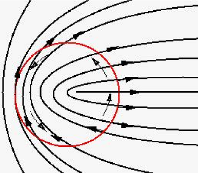
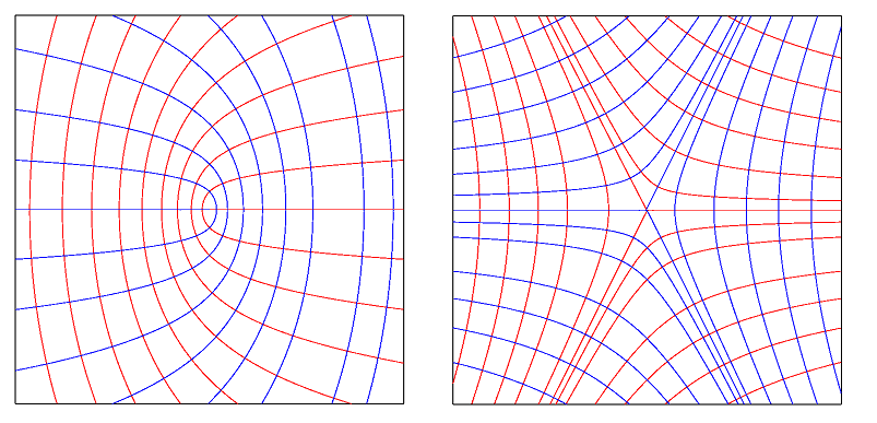
As illustrated in Figure 73.3 and Figure 73.4, the patterns made by curvature lines around an umbilic can be characterized using the notion of an index associated to the principal directions - see also [1]. As depicted in Figure 73.3, consider a small circuit \( C\) around the umbilic, and a point \( p \in C\). Starting from an initial orientation \( u\) of a tangent vector to the curvature line through point \( p\), propagate by continuity this orientation around the circuit. The index is defined by the angle swept by \( u\) around this revolution, normalized by \( 2\pi\). In our example, the index is thus 1/2.
If the index of the principal direction field is \( 1/2\) then it is called a ELLIPTIC_UMBILIC, if it is \( -1/2\) it is called a HYPERBOLIC_UMBILIC. Otherwise the umbilic is qualified NON_GENERIC_UMBILIC.
Our method aims at reporting ridges as polygonal lines living on the mesh. It assumes differential quantities are available for each vertex of the mesh (principal curvatures and directions together with third order quantities \( b_0, b_3\) and optionally fourth order quantities \( P_1, P_2\)). These differential quantities may be computed for the smooth surface the mesh is inscribed in (analytically or using approximation methods), or may be estimated for a mesh given without reference to an underlying smooth surface. Although the ridge approximation algorithm is the same in both cases, one cannot ambition to ask for the same certificates. This distinction calls for the notion of compliant mesh.
Compliant meshes.
Ridges of a smooth surface are points with prescribed differential properties, and reporting them from a mesh inscribed in the surface requires delicate hypothesis on the geometry of that mesh so as to get a certified result. In this paragraph, we assume the mesh provided complies with a number of hypothesis, which guarantee the topology of the ridges reported matches that of the ridges on the smooth surface. To summarize things, a compliant mesh is a mesh dense enough so that (i) umbilics are properly isolated (ii) ridges running next to one another are also properly separated. See [2] for a detailed discussion of compliant meshes.
As 0-level set of the extremality coefficients \( b_0\) and \( b_3\), ridges are extracted by a marching triangles algorithm.A marching triangles algorithm is similar to a 2d marching cubes algorithm (or marching rectangles algorithm), except that a one-manifold is reported on a two-manifold tessellated by triangles.
As the signs of these extremality coefficients depend on the orientation of the principal directions, we expect both extremalities and vectors orienting the principal direction to be given at each point vertex of the mesh. Except in the neighborhood of umbilics, if the mesh is dense enough, a coherent orientation of principal directions at both endpoints of an edge is chosen such that the angle between the two vectors is acute. This rule, the acute rule, is precisely analyzed in [2]. Moreover, we only seek ridges in triangles for which one can find an orientation of its three vertices such that the three edges are coherently oriented by the acute rule. Such triangles are called regular. This said, two remarks are in order.
- Regular triangles and ridge segments. A regular triangle has 0 or 2 edges crossed by a max (resp. min) ridge, which is tantamount to a sign change of \( b_0\) (resp. \( b_3\)) along the corresponding edges. In the latter case, we say that the triangle contains a ridge segment. Two methods are provided to compute its type, be it elliptic or hyperbolic. First, if fourth order differential quantities are provided, one can use the \( P_1\) ( \( P_2\)) values of Equations eqtaylor_along_line ( eqtaylor_along_red_line) for a max (min) ridge. The value of \( P_i\) for a ridge segment is defined as the mean value of the \( P_i\) values of the two crossing points on edges (while the value at a crossing point on an edge is the \( b_i\)-weighted mean value of the values at endpoints). Alternatively, if third order differential quantities only are available, one may use the geometric method developed in [2].
Using the notion of ridge segment, a Ridge_line is defined as a maximal connected sequence of ridge segments of the same type and connected together. Notice that the topology of a Ridge_line is either that of an interval or a circle.
- Non-regular triangles. In the neighborhood of umbilics, triangle are less likely to be regular and the detection of ridges cannot be relevant by this method. This is why we propose another method to detect umbilics independently.
Non compliant meshes: filtering ridges on strength and sharpness.
For real world applications dealing with coarse meshes, or meshes featuring degenerate regions or sharp features, or meshes conveying some amount of noise, the compliance hypothesis [2] cannot be met. In that case, it still makes sense to seek loci of points featuring extremality of estimated principal curvatures, but the ridges reported may require filtering. For example, if the principal curvatures are constant
The method aims at identifying some vertices of a mesh as umbilics. It assumes principal curvatures and directions are given at each vertex on the mesh.
Algorithm.
Assume each vertex \( v\) of the mesh comes with a patch (a topological disk) around it. Checking whether vertex \( v\) is an umbilic is a two stages process, which are respectively concerned with the variation of the function \( k_1-k_2\) over the patch, and the index of the vertex computed from the boundary of the patch. More precisely, vertex \( v\) is declared to be an umbilic if the following two conditions are met:
Finding patches around vertices.
Given a vertex \( v\) and a parameter \( t\), we aim at defining a collection of triangles around \( v\) so that (i) this collection defines a topological disk on the triangulation \( T\) and (ii) its size depends on \( t\). First we collect the 1-ring triangles. We define the size \( s\) of this 1-ring patch as the (Euclidean) distance from \( v\) to its farthest 1-ring vertex neighbor. We then collect recursively adjacent triangles so that the patch remains a topological disk and such that these triangles are at distance less than \( s\times t\). Parameter \( t\) is the only parameter of the algorithm.
Umbilical patches versus ridges. On a generic surface, generic umbilics are traversed by one or three ridges. For compliant meshes, an umbilic can thus be connected to the ridge points located on the boundary of its patch. This functionality is not provided, and the interested reader is referred to [2] for more details.
All classes of this package are templated by the parameter TriangleMesh, which defines the type of the mesh to which the approximation algorithms operate.
The differential quantities are provided at vertices of this mesh via property maps, a concept commonly used in the Boost library. Property maps enables the user to store scalars and vectors associated to a vertex either internally in extended vertices or externally with a std::map combined with a boost::associative_property_map.
Output of ridges or umbilics are provided via output iterators.
Approximation of ridges and umbilics are performed by two independent classes, which we now further describe.
The main class is Ridge_approximation<TriangleMesh,VertexFTMap,VertexVectorMap>. Its construction requires the mesh and the property maps defining the differential quantities for principal curvatures \( k_1\) and \( k_2\), the third order extremalities \( b_0\) and \( b_3\), the principal directions of curvature \( d_1\) and \( d_2\), and the fourth order quantities \( P_1\) and \( P_2\) if the tagging of ridges as elliptic or hyperbolic is to be done using the polynomials \( P_1\) and \( P_2\).
Three functions (provided as members and also as global functions) enable the computation of different types of ridges :
compute_max_ridges() (resp. compute_min_ridges()) outputs ridges of types MAX_ELLIPTIC_RIDGE and MAX_HYPERBOLIC_RIDGE (resp. MIN_ELLIPTIC_RIDGE and MIN_HYPERBOLIC_RIDGE). compute_crest_ridges() outputs ridges of types MAX_CREST_RIDGE and MIN_CREST_RIDGE. These functions allows the user to specify how the elliptic/hyperbolic tagging is carried out. Notice the rationale for the choice of these three functions is simple: each computation needs a single pass over the triangles of the mesh. This should be clear for the min and max ridges. For crests, just notice max and min crests cannot intersect over a triangle.
The ridge lines are stored in Ridge_line objects and output through an iterator. Each ridge line is represented as a list of halfedges of the mesh it crosses with a scalar defining the barycentric coordinate of the crossing point with respect to the half-egde endpoints. Each ridge line comes with its type Ridge_type, its strength and sharpness.
If one chooses to use only third order quantities, the quantities \( P_i\) do not have to be defined. Then the sharpness will not be defined.
The main class is Umbilic_approximation<TriangleMesh,VertexFTMap,VertexVectorMap>. Its construction requires the mesh and the property maps defining the differential quantities for principal curvatures \( k_1\) and \( k_2\), and the principal directions of curvature \( d_1\) and \( d_2\). The member function compute() (or the global function compute_umbilics()) has a parameter to define the size of the neighborhood of the umbilic.
Umbilics are stored in Umbilic objects, they come with their type : ELLIPTIC_UMBILIC, HYPERBOLIC_UMBILIC or NON_GENERIC_UMBILIC; the vertex of the mesh they are associated to and the list of half-edges representing the contour of the neighborhood.
The following program computes ridges and umbilics from an off file.Model data may be downloaded via ftp://ftp.mpi-sb.mpg.de/pub/outgoing/CGAL/Ridges_3_datafiles.tgz . The mechanical part model has been provided courtesy of Dassault System to produce Figure 73.6, due to copyright issues the available model is not the same, it is provided by the AIM@SHAPE Shape Repository. It uses the package Estimation of Local Differential Properties of Point-Sampled Surfaces to estimate the differential quantities. The default output file gives rough data for visualization purpose, a verbose output file may also be asked for. Parameters are
Monge_via_jet_fitting class, \( d\) must be greater or equal to 3 which is the default value; Monge_via_jet_fitting class, \( m\) must be 3 (the default value) or 4 and smaller than \( d\); Monge_via_jet_fitting class, in addition the number of vertices collected must be greater than \( Nd:=(d+1)(d+2)/2\) to make the approximation possible. \( a\) may be an integer greater than 1, the value 0 (which is the default) means that the minimum number of rings is collected to make the approximation possible. (Alternatively option \( p\) allows the specification of a constant number of neighbors); Ridge_order for the distinction between elliptic and hyperbolic ridges, \( t\) is 3 (default) or 4; For Figure 73.5, the data have been computed as follows:
In addition, the four elliptic umbilics are detected, the standard output being
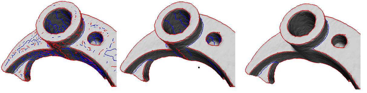
Figure 73.6 illustrates the filtering of crest ridges on a mechanical model, and has been computed as follows:
 1.8.13