|
CGAL 5.2 - Triangulated Surface Mesh Segmentation
|
|
CGAL 5.2 - Triangulated Surface Mesh Segmentation
|

Mesh segmentation is the process of decomposing a mesh into smaller and meaningful sub-meshes. This process is used in applications such as modeling, rigging, texturing, shape-retrieval, deformation ... We refer to a comprehensive survey on mesh segmentation [3] for different segmentation techniques.
This package provides an implementation of the algorithm relying on the Shape Diameter Function [4] (SDF). Given a triangulated surface mesh (simply mesh in the following) bounding a 3D solid object, the SDF provides an estimate of the local object diameter for each facet of the mesh (the SDF values). The segmentation algorithm first applies a soft clustering on the facets using the associated SDF values. The final segmentation is then obtained via a graph-cut algorithm that considers surface-based features (dihedral-angle and concavity) together with the result of the soft clustering.
This package offers the computation of the SDF values and the mesh segmentation result as independent functions. This allows an alternative implementation of the SDF to be directly plugged into the segmentation algorithm, and also to reuse the SDF values several times with different parameters for the segmentation algorithm.
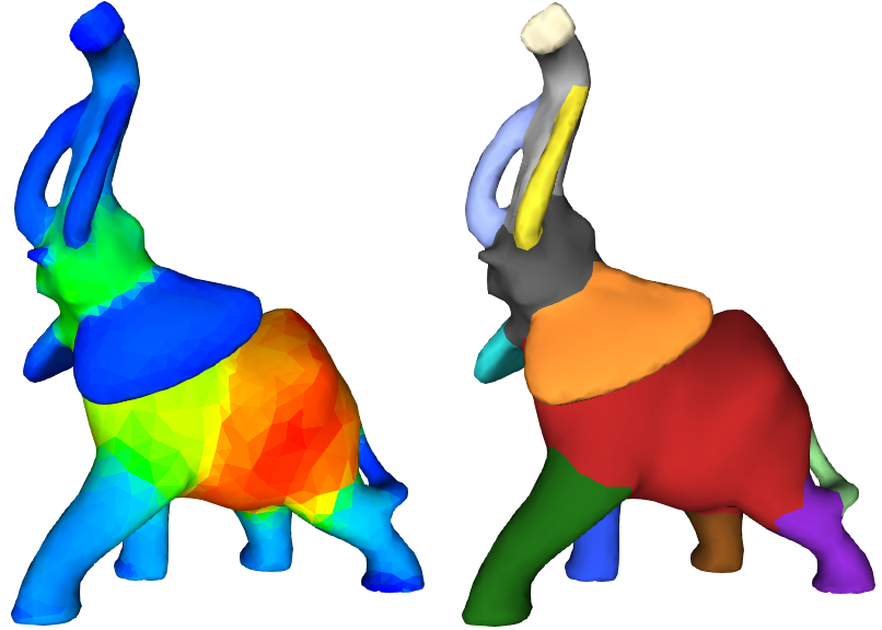
The Shape Diameter Function provides a connection between the surface mesh and the volume of the subtended 3D bounded object. More specifically, the SDF is a scalar-valued function defined on facets of the mesh that measures the corresponding local object diameter. The SDF is used to distinguish between thin and thick parts by adding a local notion of thickness to the facets. In addition, the SDF is pose-invariant: SDF values remain largely unaffected after changes of pose (see Figure 67.2).

For a given input mesh, the raw SDF values are computed by processing each facet one by one. For each facet, several rays are sampled in a cone constructed using the centroid of the facet as apex and inward-normal of the facet as axis. Each ray is truncated into a segment, its endpoints being the apex of the cone and the first mesh facet intersection point. Using the lengths of these truncated rays, which intuitively correspond to a local volume sampling, the raw SDF value is computed by first applying an outlier removal procedure and then taking the average of the lengths.
The raw SDF values are computed through function sdf_values(), setting postprocess to false.
After having calculated the raw SDF value for each facet, the SDF values used in the segmentation algorithm are the result of several post-processing steps:
segmentation_from_sdf_values().A bilateral smoothing [5] is applied. This smoothing technique removes the noise while trying to keep fast changes on SDF values unchanged since they are natural candidates for segment boundaries. The bilateral smoothing [5] has three parameters that are set as follows:
Large window sizes are more effective at eliminating noise but may over-smooth SDF values along segment boundaries. Large range parameters make smoothing closer to Gaussian smoothing and may also lead to over-smoothed SDF values.
These post-processing steps can be applied to raw SDF values (or an alternative set of similar scalar values associated with facets) using the function sdf_values_postprocessing().
Given a number \( k \) of clusters, the soft clustering is a Gaussian mixture model that consists in fitting \( k \) Gaussian distributions to the distribution of the SDF values of the facets. It is initialized with k-means++ [1], and run multiple times with random seeds. Among these runs, the best result is used for initializing the expectation-maximization algorithm for fitting the Gaussian distributions.

The output of this procedure is a matrix that contains probability values for each facet to belong to each cluster. These probability values are used as input to the hard clustering.
The hard clustering yields the final segmentation of the input mesh and results from minimizing an energy function combining the aforementioned probability matrix and geometric surface features.
The energy function minimized using alpha-expansion graph cut algorithm [2] is defined as follows:
\( E(\bar{x}) = \sum\limits_{f \in F} e_1(f, x_f) + \lambda \sum\limits_{ \{f,g\} \in N} e_2(x_f, x_g) \) \( e_1(f, x_f) = -log(max(P(f|x_f), \epsilon)) \) \( e_2(x_f, x_g) = \left \{ \begin{array}{rl} -log(\theta(f,g)/\pi) &\mbox{ $x_f \ne x_g$} \\ 0 &\mbox{ $x_f = x_g$} \end{array} \right \} \) | where:
|
The first term of the energy function provides the contribution of the soft clustering probabilities. The second term of the energy function is a geometric criterion that is larger when two adjacent facets sharing a sharp and concave edge are in the same cluster. The smoothness parameter makes this geometric criteria more or less prevalent.
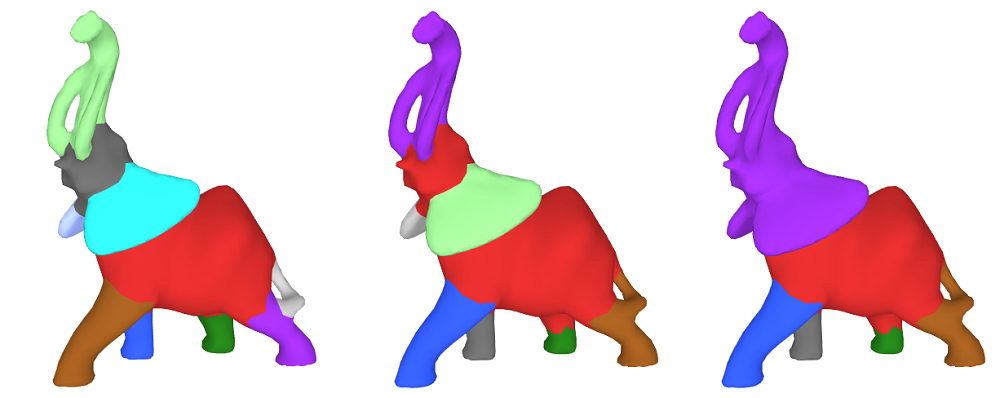
Assigning a high value to the smoothness parameter results in a small number of segments (since constructing a segment boundary would be expensive). In other words, merging facets that are placed under different clusters is less expensive than separating them and creating boundaries. On the contrary, assigning smaller values to smoothness parameter results in a high number of segments, by getting closer to the result of the soft clustering (notice that setting \( \lambda=0 \) provides the result of the soft clustering). Figure 67.4 depicts the influence of the smoothness parameter.

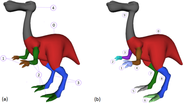
The hard clustering assigns a cluster id to each facet (see Figure 67.5 (a)). A segment consists in a set of connected facets in the same cluster (see Figure 67.5 (b)). By default the function segmentation_from_sdf_values() assigns to each facet the id of its segment. It assigns to each facet the id of its cluster when output_cluster_ids is set to true.

Four functions are provided:
sdf_values() : computes the SDF value of each facet of an input mesh in either raw or post-processed form. SDF values are associated to facets using a property map (see CGAL and Boost Property Maps).sdf_values_postprocessing() : post-processes raw SDF values. The post-processing is decoupled from the function sdf_values() to allow the use of alternative methods to compute SDF values or additional post-processing step.segmentation_from_sdf_values() : computes the mesh segmentation from the SDF values of the facets of an input mesh. The input SDF values can be any set of scalar values associated to each facet as long as they have been normalized between 0 and 1. This function allows using the same SDF values with different parameters for the segmentation stage. The segment or cluster ids are associated to the facets using a property map.segmentation_via_sdf_values() : combines the three functions above.These functions expect as input a triangulated surface mesh bounding a 3D solid object, with the following properties:
The current implementation of the computation of the SDF values relies on the 3D Fast Intersection and Distance Computation package. This operation is reliable when the AABBTraits model provided has exact predicates. CGAL::Exact_predicates_inexact_constructions_kernel is recommended as geometric traits for this algorithm.
File Surface_mesh_segmentation/sdf_values_example.cpp
File Surface_mesh_segmentation/segmentation_from_sdf_values_example.cpp
The function segmentation_via_sdf_values() combines the computation of sdf values, the post-processing and the segmentation. Note that when computing several segmentations of a mesh with different parameters (i.e. number of levels, and smoothing lambda), it is advised to first compute the SDF values using sdf_values() and use them in calls of the function segmentation_from_sdf_values().
File Surface_mesh_segmentation/segmentation_via_sdf_values_example.cpp
The previous examples use a std::map as property maps for storing the SDF values and the segmentation results. This example uses a polyhedron type with a facet type storing an extra ID field, together with a vector, as underlying data structure in the property maps. The main advantage is to decrease from log to constant the complexity for accessing the data associated to facets.
File Surface_mesh_segmentation/segmentation_with_facet_ids_example.cpp
When using a Surface_mesh, you can use the built-in property mechanism.
File Surface_mesh_segmentation/segmentation_from_sdf_values_SM_example.cpp
It is possible to consider each segment as an independent triangle mesh, like in the following example, where the area of each segment is computed.
File Surface_mesh_segmentation/extract_segmentation_into_mesh_example.cpp
The following tables provide the runtime of the functions sdf_values() and segmentation_from_sdf_values(). The results were produced with the release 4.4 of CGAL, on an Intel i7 3.2 Ghz laptop with 8 GB RAM, compiled by Visual C++ 2010 with /O2 option. The polyhedron types are using Polyhedron_items_with_id_3 as item class. The models used for the benchmarks are the dinosaur model with 7,828 facets, the bear model with 20,188 facets and the elephant model with 88,928 facets.
Runtime in seconds of sdf_values() with 25 rays showing the cost of the robustness:
| Number of triangles | Simple_cartesian<double> | Exact_predicates_inexact_constructions_kernel (EPICK) |
|---|---|---|
| 7,828 | 2.3 | 3.8 |
| 20,188 | 6.1 | 9.5 |
| 88,928 | 46.1 | 62.3 |
Runtime in milliseconds of segmentation_from_sdf_values() (using Simple_cartesian<double> or EPICK gives the same results), the graph-cut part is using the library MaxFlow v2.21:
| Number of triangles | Number of cluster = 2 | Number of cluster = 5 | Number of cluster = 10 | Number of cluster = 15 |
|---|---|---|---|---|
| 7,828 | 38 | 61 | 141 | 204 |
| 20,188 | 50 | 163 | 483 | 608 |
| 88,928 | 314 | 1,260 | 2,736 | 4,239 |
The initial implementation of this package is the result of the work of Ilker O. Yaz during the 2012 season of the Google Summer of Code. He has been mentored by Sébastien Loriot who also contributed to the documentation and the API definition.