|
CGAL 5.2.1 - Shape Detection
|
|
CGAL 5.2.1 - Shape Detection
|
This CGAL component implements two algorithms for shape detection:
From an unstructured point set with unoriented normals, this algorithm detects a set of shapes (see Figure Figure 78.1). Five types of primitive shapes are provided by this package: plane, sphere, cylinder, cone, and torus. Other primitive shapes can be easily added by the user (see Section Custom Shapes).
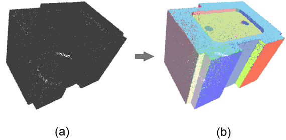
This method takes as input a point set with unoriented normals and provides as output a set of detected shapes with associated input points. The output of the algorithm is a set of detected shapes with assigned points and all remaining points not covered by these shapes. Each input point can be assigned to at most one detected shape.
The shapes are detected via a RANSAC-type approach, that is a random sample consensus. The basic RANSAC approach repeats the following steps:
Steps 1-3 are repeated for a prescribed number of iterations and the shape with the highest number of inliers, referred to as the largest shape, is kept.
In our context, the error between a point and a shape is defined by its distance and normal deviation to the shape. A random subset corresponds to the minimum number of points (with normals) required to uniquely define a primitive.
For very large point sets, the basic RANSAC method is not practical when testing all possible shape candidates against the input data in order to find the largest shape. The main idea behind the Efficient RANSAC method is testing shape candidates against subsets of the input data. Shape candidates are constructed until the probability to miss the largest candidate is lower than a user-specified threshold. The largest shape is repeatedly extracted until no more shapes, restricted to cover a minimum number of points, can be extracted. An additional gain in efficiency is achieved through exploiting the normal attributes during initial shape construction and enumeration of inliers.
The support of a shape refers to the footprint of the points covered by the primitive. To avoid generating shapes with the fragmented support, we enforce a connectivity constraint by considering only one connected component, referred to as cluster, selected as the one covering the largest number of inliers (see Section Parameters for more details).
The algorithm has five parameters:
epsilon and normal_threshold: The error between a point-with-normal \(p\) and a shape \(S\) is defined by its Euclidean distance and normal deviation to \(S\). The normal deviation is computed between the normal at \(p\) and the normal of \(S\) at the closest projection of \(p\) onto \(S\). The parameter epsilon defines the absolute maximum tolerance Euclidean distance between a point and a shape. A high value of epsilon leads to the detection of fewer large shapes and hence a less detailed detection. A low value of epsilon yields a more detailed detection, but may lead to either lower coverage or over-segmentation. Over-segmentation translates into detection of fragmented shapes when epsilon is within or below the noise level. When the input point set is made of free-form parts, a higher tolerance epsilon enables to detect more primitive shapes that approximate some of the free-form surfaces. The impact of this parameter is depicted by Figure Figure 78.2. Its impact on performance is evaluated in Section Performance.
epsilon set to 2.0 (one color per detected shape). Most details such as chimneys on the roof are not distinguished. (c) Detection with epsilon set to 0.5. The facades are correctly detected and some details of the roof are detected. (d) Setting epsilon to 0.25 yields a more detailed but slightly over-segmented detection. cluster_epsilon: The Efficient RANSAC uses this parameter to cluster the points into connected components covered by a detected shape. For developable shapes that admit a trivial planar parameterization (plane, cylinder, cone), the points covered by a shape are mapped to a 2D parameter space chosen to minimize distortion and best preserve arc-length distances. This 2D parameter space is discretized using a regular grid, and a connected component search is performed to identify the largest cluster. The parameter cluster_epsilon defines the spacing between two cells of the regular grid, so that two points separated by a distance of at most \(2\sqrt{2}\) cluster_epsilon are considered adjacent. For non-developable shapes, the connected components are identified by computing a neighboring graph in 3D and walking in the graph. The impact of the parameter cluster_epsilon is depicted in Figure Figure 78.3.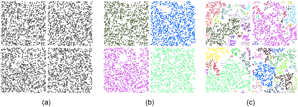
cluster_epsilon controls the connectivity of the points covered by a detected shape. The input point set is sampled on four coplanar squares. (a) A large value of cluster_epsilon leads to detecting a single planar shape. (b) A moderate value of cluster_epsilon yields the detection of four squares. Notice that a few points within the squares are not detected as not connected. (c) A small value of cluster_epsilon leads to over-segmentation. min_points: The minimum number of points controls the termination of the algorithm. The shape search is iterated until no further shapes can be found with a higher support. Note that this parameter is not strict: depending on the chosen probability, shapes may be extracted with a number of points lower than the specified parameter.probability: This parameter defines the probability to miss the largest candidate shape. A lower probability provides a higher reliability and determinism at the cost of longer running time due to a higher search endurance.The main class Shape_detection::Efficient_RANSAC takes a template parameter Shape_detection::Efficient_RANSAC_traits that defines the geometric types and input format. Property maps provide a means to interface with the user-specific data structures. The first parameter of the Shape_detection::Efficient_RANSAC_traits class is the common Kernel. In order to match the constraints of property maps, an iterator type and two maps that map an iterator to a point and a normal are specified in the Shape_detection::Efficient_RANSAC_traits class. The concept behind property maps is detailed in Manual CGAL and Property Maps.
Typical usage consists of five steps:
The following example reads a point set from a file and detects only planar shapes. The default parameters are used for detection.
File Shape_detection/efficient_RANSAC_basic.cpp
The Efficient RANSAC class provides a callback mechanism that enables the user to track the progress of the algorithm. It can be used, for example, to terminate the algorithm based on a timeout. In the following example, the algorithm stops if it takes more than half a second and prints out the progress made.
File Shape_detection/efficient_RANSAC_with_callback.cpp
This example illustrates the user selection of parameters using the Shape_detection::Efficient_RANSAC::Parameters class. Shape detection is performed on five shape types (plane, cylinder, sphere, cone, and torus). The input point set is sampled on a surface mostly composed of piecewise planar and cylindrical parts, in addition to free-form parts.
Basic information of the detected shapes is written to the standard output: if the shape is either a plane or a cylinder, specific parameters are recovered, otherwise the general method info() is used to get the shape parameters in a string object. Note that specific parameters can be recovered for any of the provided shapes.
File Shape_detection/efficient_RANSAC_with_parameters.cpp
This example illustrates how to access the points assigned to each shape and compute the mean error. A timer measures the running performance.
File Shape_detection/efficient_RANSAC_with_point_access.cpp
Other shape types can be detected by implementing a shape class derived from the class Shape_detection::Shape_base and registering it to the shape detection factory of the Efficient RANSAC object. This class must provide the following functions: construct a shape from a small set of given points, compute the squared distance from a query point to the shape, and compute the normal deviation between a query point with the normal and the normal to the shape at the closest point from the query. The used shape parameters are added as members to the derived class.
Note that the RANSAC approach is efficient for shapes that are uniquely defined by a small number of points, denoted by the number of required samples. The algorithm aims at detecting the largest shape via many random samples, and the combinatorial complexity of possible samples increases rapidly with the number of required samples.
More specifically, the functions to be implemented are defined in the base class Shape_detection::Shape_base:
Shape_detection::Shape_base::minimum_sample_size() const: Returns the minimum number of required samples.Shape_detection::Shape_base::create_shape(const std::vector<size_t>& indices): The randomly generated samples are provided via a vector of indices. Shape_detection::Shape_base::point(std::size_t index) and Shape_detection::Shape_base::normal(std::size_t index) are used to retrieve the actual points and normals (see the example below). The provided number of samples might actually be larger than the above minimum number of required samples, depending on the other shape types. If the provided samples are not sufficient to define a unique shape, for example in a degenerated case, the shape is considered invalid.Shape_detection::Shape_base::squared_distance(const Point& point) const: This function computes the squared distance from a query point to the shape. It is used for traversing the hierarchical spatial data structure.Shape_detection::Shape_base::squared_distance(std::vector<FT>& distances, const std::vector<size_t>& indices) andShape_detection::Shape_base::cos_to_normal(const std::vector<size_t>& indices, std::vector<FT>& angles) const.The last two functions are used to determine the number of inlier points to the shape. They compute respectively the squared distance from a set of points to the shape, and the dot product between the point normals and the normals at the shape for the closest points on the shape.
The access to the actual point and normal data is carried out via Shape_detection::Shape_base::point(std::size_t index) and Shape_detection::Shape_base::normal(std::size_t index) (see the example below). The resulting squared distance/dot product is stored in the vector provided as the first argument.
By default, the connected component is detected via the neighbor graph as mentioned above. However, for shapes that admit a faster approach to detect a connected component, the user can provide his/her own implementation to extract the connected component via:
Shape_detection::Shape_base::connected_component(std::vector<std::size_t>& indices, FT cluster_epsilon): The indices of all supporting points are stored in the vector indices. All points that do not belong to the largest cluster of points are removed from the vector indices.Another optional method can be implemented to provide a helper function providing the shape parameters written to a string:
Shape_detection::Shape_base::info(): This function returns a string suitable for printing the shape parameters into a log/console. The default solution provides an empty string.The property maps are used to map the indices to the corresponding points and normals. The following header shows an implementation of a planar shape primitive, which is used by the example Shape_detection/efficient_RANSAC_with_custom_shape.cpp.
File Shape_detection/include/efficient_RANSAC_with_custom_shape.h
The running time and detection performance of the Efficient RANSAC depend on the chosen parameters. A selective error tolerance parameter leads to higher running time and fewer shapes, as many shape candidates are generated to find the largest shape. We plot the detection performance against the epsilon error tolerance parameter for detecting planes in a complex scene with 5M points (see Figure Figure 78.4). The probability parameter controls the endurance when searching for the largest candidate at each iteration. It barely impacts the number of detected shapes, has a moderate impact on the size of the detected shapes, and increases the running time. We plot the performance against the probability parameter (see Figure Figure 78.5).
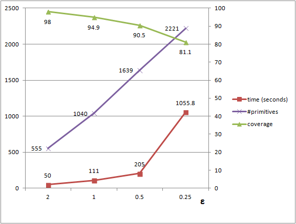
epsilon tolerance parameter. A higher value for epsilon, that is a more tolerant error, leads to fewer but larger shapes and shorter running times. 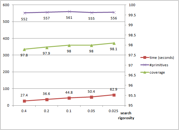
probability to miss the largest shape at each iteration. The number of shapes is stable and the coverage increases when the probability is lowered. The running time increases significantly as many more candidates are generated during each iteration of the algorithm. This shape detection component is based on the region growing algorithm applied to a set of user-specified items. Shapes are detected by growing regions from seed items, where each region is created as follows:
Together with the generic algorithm's implementation CGAL::Shape_detection::Region_growing, three particular instances of this algorithm are provided:
Other instances can be easily added by the user, as explained below.
The main class CGAL::Shape_detection::Region_growing is parameterized by
InputRange that stores a range of user-defined input items;Using this generic framework, users can grow any type of regions on a set of arbitrary items with their own propagation and seeding conditions (see an example).
The concept NeighborQuery provides the means for accessing neighbors of an item. To create a model that respects this concept, the user has to provide an overload of the operator:
NeighborQuery::operator()() that has to fill a vector with indices of all items, which are neighbors of the query item.The concept RegionType provides the means for validating regions. In fact, a model of this concept maintains a description of the region type that is used in region growing. To create a model that respect this concept, three functions have to be defined:
RegionType::is_part_of_region() This function checks if an item satisfies all necessary region requirements and can be added to a region. It is called per item.RegionType::is_valid_region() This function checks if a region satisfies all necessary region requirements. It is called per region.RegionType::update() This utility function enables to update any information, which is maintained with the region.The SeedMap property map, provided as an optional parameter to the main class, enables to define the seeding order of items that is which items are used first to grow regions from. Such items are referred to as seed items. The SeedMap maps the index of an item to its order number in the overall region growing processing queue. The default map is the identity one that is the seed index of the item equals to the item's index in the input_range. If it maps to std::size_t(-1), then the corresponding item is skipped.
This toy example shows how to define one's own NeighborQuery and RegionType classes, which are used to parameterize the CGAL::Shape_detection::Region_growing. It also shows how to skip unnecessary items and change their default seeding order.
We choose a simple custom object item. We define four such objects, where for each object, we manually store indices of its neighbors. The operator NeighborQuery::operator()() does nothing but accessing these neighbors. The RegionType class defines the three necessary functions:
RegionType::is_part_of_region() - true if the first and second objects are neighbors,RegionType::is_valid_region() - always true after the first call to the function update(),RegionType::update() - updates the internal flag from the default false to true.We also define a SeedMap, such that the second object is handled first, while the first object follows. Moreover, the last object is always skipped. Notice that in this example, the container with objects is std::vector, which is random access. However, the generic region growing algorithm can be applied to any other type of container, e.g. std::list.
The result of using these classes with the region growing main class is that the first two objects form the first region, the third object forms the second region, and the last object is skipped.
File Shape_detection/region_growing_with_custom_classes.cpp
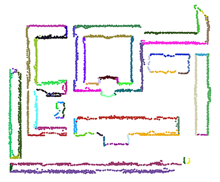
If one wants to detect lines (see 2D Example)
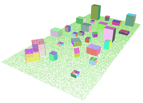
or planes (see 3D Example)
in a 2D or 3D point set respectively, this CGAL component provides the corresponding models of the concepts NeighborQuery and RegionType. In particular, it provides two different ways to define neighbors of a point:
CGAL::Shape_detection::Point_set::Sphere_neighbor_query. This class creates a circle (in 2D case) or a sphere (in 3D case) centered at the query point with a user-specified sphere radius. All points, which belong to the sphere, will be treated as neighbors of the query point;CGAL::Shape_detection::Point_set::K_neighbor_query. This class finds K (specified by the user) nearest neighbors of the query point either 2D or 3D.The component also provides
CGAL::Shape_detection::Point_set::Least_squares_line_fit_region - least squares line fit type of region for 2D points;CGAL::Shape_detection::Point_set::Least_squares_plane_fit_region - least squares plane fit type of region for 3D points.The program associates all points from a region to the best-fit hyperplane (2D line or 3D plane) and controls the quality of this fit.
The quality of region growing in a point set (2D or 3D) can be improved by slightly sacrificing the running time. To achieve this, one can sort indices of input points with respect to some quality criteria. These quality criteria can be included through the SeedMap input parameter. We provide a quality sorting both for 2D and 3D points:
CGAL::Shape_detection::Point_set::Least_squares_line_fit_sorting - indices of 2D input points are sorted with respect to the quality of the least squares line fit applied to the neighbors of each point;CGAL::Shape_detection::Point_set::Least_squares_plane_fit_sorting - indices of 3D input points are sorted with respect to the quality of the least squares plane fit applied to the neighbors of each point.The classes in Section Region Growing On Point Set depend on a few parameters that should be defined by the user. They also have default values, but these values do not necessarily guarantee to produce pleasant results.
The NeighborQuery related classes depend on the following parameters:
sphere_radius is used by the class CGAL::Shape_detection::Point_set::Sphere_neighbor_query and defines the radius of the fuzzy search sphere centered at the query point;k is used by the class CGAL::Shape_detection::Point_set::K_neighbor_query and defines the number K of nearest neighbors of the query point.The right choice of sphere_radius or k parameters plays an important role in producing a good result. For example, if we consider the fuzzy sphere neighborhood, when sphere_radius is too large, we have fewer regions, and the details are not clearly separated. Meanwhile, if sphere_radius is too small, we produce more regions, and the point set may be over-segmented. Consider a 2D map of an intersection of streets in a city as in Figure Figure 78.8. Each region is painted with a unique color. As sphere_radius increases, the details become less clear. When sphere_radius = 0.3 (c), the best visual result is produced.
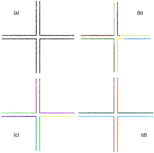
sphere_radius = 0.1; (c) 8 regions are found when sphere_radius = 0.3; (d) 4 regions are found when sphere_radius = 1.2. The RegionType related classes depend on the following parameters:
distance_threshold - the maximum distance from a point to a line/plane;angle_threshold - the maximum accepted angle between the normal associated with a point and the normal of a line/plane;min_region_size - the minimum number of points a region must have.The first two parameters are used by the functions RegionType::is_part_of_region() and RegionType::update(), while the third parameter is used by the function RegionType::is_valid_region() explained in Section Framework Region Type.
The right choice of distance_threshold and angle_threshold parameters is also very important. For example, Figure Figure 78.9 shows that the roof top of the house can be distinguished as two planes (painted in blue and dark red) when angle_threshold is strict enough (c), or it can be recognized as only one plane (painted in pale yellow) in the other case (b).
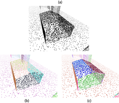
angle_threshold = 60 degrees; (c) Result when angle_threshold = 25 degrees. Typical usage of the Region Growing component consists of five steps:
NeighborQuery and RegionType with the proper parameters;CGAL::Shape_detection::Region_growing;Given a 2D point set, we detect 2D lines using the fuzzy sphere neighborhood. We then color all points from the found regions and save them in a file (see Figure Figure 78.6).
The points with assigned to them normal vectors are stored in std::vector and the used Kernel is CGAL::Simple_cartesian, where the number type is double.
File Shape_detection/region_growing_on_point_set_2.cpp
If we are given a 3D point set, then the example below shows how to detect 3D planes using the K nearest neighbors search. We color all points from the found regions and save them in a file (see Figure Figure 78.7). The example also shows how to retrieve all points, which are not assigned to any region, and how to use a custom output iterator.
The point set with associated normals is stored in CGAL::Point_set_3 and the used Kernel is CGAL::Exact_predicates_inexact_constructions_kernel.
File Shape_detection/region_growing_on_point_set_3.cpp
The main parameter that affects the region growing algorithm on a point set is the neighborhood size at each retrieval (sphere_radius or k). Larger neighbor lists are often followed by a smaller number of regions, larger coverage (the ratio between the number of points assigned to regions and the total number of input points), and longer running time. For example, for a test of about 70k 2D points with the fuzzy sphere neighborhood, the following table is produced:
sphere_radius | Time (in seconds) | Number of regions | Number of assigned points |
|---|---|---|---|
| 1 | 0.138831 | 794 | 4483 |
| 3 | 0.069098 | 3063 | 63038 |
| 6 | 0.077703 | 2508 | 64906 |
| 9 | 0.093415 | 2302 | 65334 |
If the neighborhood size is set too low, some points might be isolated, the region size would not reach a critical mass and so will be discarded. This does not only cause the latency in the program, but also reduces the coverage value, as can be seen when the sphere_radius = 1. A typical time measure for a 3D point set with the K nearest neighborhood and well-defined parameters can be found in the following table:
Number of points | Time (in seconds) |
|---|---|
| 300k | 0.761617 |
| 600k | 1.68735 |
| 900k | 2.80346 |
| 1200k | 4.06246 |
If one wants to detect planes on a polygon mesh, this CGAL component provides the corresponding models of the concepts NeighborQuery and RegionType. In particular, it has
CGAL::Shape_detection::Polygon_mesh::One_ring_neighbor_query class that retrieves all edge-adjacent faces of a face, andCGAL::Shape_detection::Polygon_mesh::Least_squares_plane_fit_region class that fits a 3D plane to the vertices of all mesh faces, which have been added to the region so far, and controls the quality of this fit.This component accepts any model of the concept FaceListGraph as a polygon mesh. A picture below gives an example of the region growing algorithm for detecting 3D planes on CGAL::Surface_mesh.
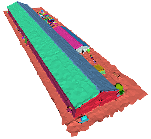
The quality of region growing on a polygon mesh can be improved by slightly sacrificing the running time. To achieve this, one can sort indices of input faces with respect to some quality criteria. These quality criteria can be included in region growing through the SeedMap input parameter. We provide such a quality sorting:
CGAL::Shape_detection::Polygon_mesh::Least_squares_plane_fit_sorting - indices of input faces are sorted with respect to the quality of the least squares plane fit applied to the neighbors of each face.The NeighborQuery related class does not require any parameters, because edge-adjacent faces are found using the internal face graph connectivity, while the RegionType related class depends on three parameters:
distance_threshold - the maximum distance from the furthest face vertex to a plane;angle_threshold - the maximum accepted angle between the face normal and the normal of a plane;min_region_size - the minimum number of mesh faces a region must have.The first two parameters are used by the functions RegionType::is_part_of_region() and RegionType::update(), while the third parameter is used by the function RegionType::is_valid_region() explained in Section Framework Regions. The right choice of these parameters is as important as the one explained in Section Parameters For Region Growing On Point Set.
In the example below, we show how to use region growing to detect planes on a polygon mesh that can be either stored as CGAL::Surface_mesh or CGAL::Polyhedron_3. If it is a surface mesh, this example also provides a way to save the result in a file (see Figure Figure 78.10). The used Kernel here is CGAL::Exact_predicates_exact_constructions_kernel. Though this exact kernel provides better quality results, please note that it may significantly slow down the execution of the program, so if you need a faster version of region growing, use a floating type based kernel.
We can improve the quality of region growing by providing a different seeding order (analogously to Point Sets) that is why in this example we also sort indices of input faces using the CGAL::Shape_detection::Polygon_mesh::Least_squares_plane_fit_sorting and only then detect regions.
File Shape_detection/region_growing_on_polygon_mesh.cpp
Since accessing neighbors of a face in a polygon mesh is fast, performance of the region growing on a polygon mesh mostly depends on the RegionType model's implementation, which is usually fast, too.
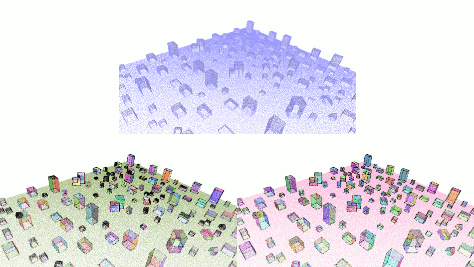
The Efficient RANSAC algorithm is very quick, however, since it is not deterministic, some small shapes might be missed in the detection process.
Instead, the region growing algorithm usually takes longer to complete, but it may provide better quality output in the presence of large scenes with numerous small details. Since it iterates throughout all items of the scene, there are fewer chances to miss a shape. In addition, it is deterministic (for a given input and a given set of parameters, it always returns the same output, whereas the Efficient RANSAC algorithm is randomized and so the output may vary at each run), see Figure Figure 78.11.
Shape detection applies to man-made scenes or objects such as urban scenes or scans of mechanical parts. Such scenes often contain a wide range of geometric regularities such as parallelism, orthogonality, or symmetry. This package offers a function to reinforce four types of regularities for planar shapes, CGAL::regularize_planes():
The user can choose to regularize only one or several of these four properties (see Reference Manual). The process is greedy and based on a hierarchical decomposition (coplanar clusters are subgroups of parallel clusters, which are subgroups of axis-symmetric and orthogonal clusters) as described by Verdie et al. [3]
File Shape_detection/efficient_RANSAC_and_plane_regularization.cpp
The new version (see all examples above) of the class CGAL::Shape_detection::Region_growing is not compatible with the old API. For the old API, see an example below and use CGAL::Shape_detection::deprecated::Region_growing_depr instead.
File Shape_detection/shape_detection_basic_deprecated.cpp
The old API is still supported, but will be removed in the next releases. In particular, the classes CGAL::Shape_detection::deprecated::Region_growing_depr and CGAL::Shape_detection::deprecated::Shape_detection_traits will be removed. Please update your code.
The Efficient RANSAC component was developed by Sven Oesau based on the prototype version created by Yannick Verdie, with the help of Clément Jamin and under the supervision of Pierre Alliez. Plane regularization was added by Simon Giraudot based on the prototype version developed by Florent Lafarge.
The region growing algorithm on a 3D point set was first implemented by Simon Giraudot based on the prototype version developed by Florent Lafarge and then generalized to arbitrary items including versions for a 2D point set, a 3D point set, and a polygon mesh by Thien Hoang during the Google Summer of Code 2018 under the supervision of Dmitry Anisimov.
The authors wish to thank our reviewers Andreas Fabri, Sébastien Loriot, and Simon Giraudot for helpful comments and discussions.