

|
CGAL 5.2.4 - 3D Spherical Geometry Kernel
|
|
CGAL 5.2.4 - 3D Spherical Geometry Kernel
|
The goal of the 3D spherical kernel is to offer to the user a large set of functionalities on spheres, circles and circular arcs, in the 3D space or restricted on a given sphere. These functionalities require computing on algebraic numbers, which motivates the creation of a new kernel concept extending the CGAL Kernel concept, that is restricted to objects and functionality in a FieldNumberType.
All the choices (interface, robustness, representation, and so on) made here are consistent with the choices made in the CGAL kernel, for which we refer the user to the 2D and 3D Linear Kernel).
New main geometric objects are introduced by Spherical_kernel_3: circular arcs ((model of SphericalKernel::CircularArc_3), points of circular arcs (model of SphericalKernel::CircularArcPoint_3), and line segments (model of SphericalKernel::LineArc_3) whose endpoints are points of this new type.
SphericalKernel::CircularArcPoint_3 is used in particular for endpoints of arcs and intersection points between spheres, circles or arcs. The coordinates of these points are algebraic numbers of degree two. Therefore, general predicates offered by the Kernel on Point_3, which have coordinates in a FieldNumberType, would require heavy algebraic computations in algebraic extensions of higher degrees and thus are not provided on them, which explains the need for a new point type.
A consistent set of predicates and constructions is offered on these new types.
General Functionalities
The spherical kernel currently implements a set of fundamental functionalities like intersection, comparisons, inclusion, etc. More might be provided in the future, as long as only algebraic numbers of degree two are used.
Functionalities Relative to a Sphere
The interface of the underlying objects is extended by providing additional operations that make sense only if the objects are considered on the same sphere. For example, the result of the comparison of the cylindrical or spherical coordinates of two points is well-defined only when looking at them on a given common sphere. The presentation of these operations requires the following definitions:
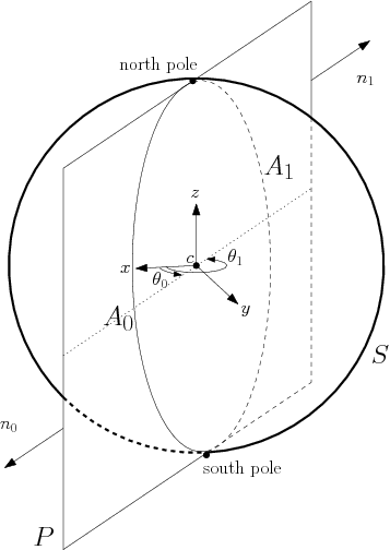
Coordinate system. Let consider a sphere with center c and radius r. Using the Cartesian frame centered at c, we define a cylindrical coordinate system \( (\theta,z)\) on that sphere, with \( \theta \in \left[ 0,2\pi \right)\) and \( z \in \left[ -r,r \right]\). \( \theta\) is given in radian and measured in the \( xy\)-plane around the \( z\)-axis, starting from \( x>0\), \( y=0\). The \( z\)-extremal points of a sphere are its North and South poles defined as \( (\theta,r)\) and \( (\theta,-r)\) respectively, for any value of \( \theta\). Observe that each point on the sphere different from a pole corresponds to a unique pair \( (\theta,z)\).
Definition of a meridian. Given a sphere and its associated cylindrical coordinate system, a meridian of that sphere is a circular arc consisting of the points having the same theta-coordinate (the poles are the end points). A plane containing the two poles of that sphere defines two meridians, one on each side of the line passing through the poles. A vector \( M\) whose direction is different from that of the latter line defines a unique meridian on that sphere. The plane of that meridian is defined by the direction of \( M\) and the two poles. The sense of \( M\) disambiguates the choice among the pair of meridians thus defined. On Figure 11.1, the normal vectors \( n_0\) and \( n_1\) define two meridians of \( S\): the circular arcs \( A_0\) and \( A_1\) respectively.
Types of circles on a sphere. Given a sphere, a circle on that sphere is termed polar if it goes through only one pole, bipolar if it goes through the two poles of that sphere and threaded if it separates the sphere into two connected components, each containing one pole. Any other circle is termed normal. These definitions are illustrated on Figure 11.2.
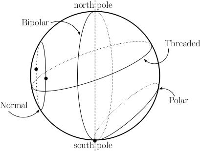
\( \theta\)-extremal points. Given a sphere one has: a \( \theta\)-extremal point of a normal circle is a point of tangency between the circle and a meridian anchored at the poles of that sphere. Each normal circle defines two such points; the \( \theta\)-extremal point of a polar circle is the pole the circle goes through. No such point is defined on a bipolar or a threaded circle. These definitions are illustrated on Figure 11.2. Notice that the \( \theta\)-extremal points should not be confused with the endpoints of an arbitrary arc on a sphere.
The \( \theta\)-coordinate of a \( \theta\)-extremal point of a normal circle on a sphere is well defined. For a polar circle on a sphere, the plane containing the two poles and which is tangent to that circle contains two different meridians. The \( \theta\)-values of these meridians are the two \( \theta\)-coordinates associated to the same \( \theta\)-extremal point of a polar circle.
\( \theta\)-monotone circular arcs. An arc on a sphere is said to be \( \theta\)-monotone if any meridian on that sphere intersects that arc in at most one point. With this definition, a circular arc on a threaded circle is always \( \theta\)-monotone, and an arc on a polar or normal circle is \( \theta\)-monotone if it does not contain a \( \theta\)-extremal point, unless it is an endpoint. No such arc is defined on a bipolar circle.
The design of Spherical_kernel_3 is similar to the design of Circular_kernel_2 (see Chapter 2D Circular Geometry Kernel).
It has two template parameters:
Kernel concept. The spherical kernel derives from it, and it provides all elementary geometric objects like points, lines, spheres, circles and elementary functionality on them. AlgebraicKernelForSpheres. The robustness of the package relies on the fact that the algebraic kernel provides exact computations on algebraic objects. The 3D spherical kernel uses the extensibility scheme presented in the kernel manual (see Section Extensible Kernel). The types of Kernel are inherited by the 3D spherical kernel and some types are taken from the AlgebraicKernelForSpheres parameter. Spherical_kernel_3 introduces new geometric objects as mentioned in Section Spherical Kernel Objects.
In fact, the spherical kernel is documented as a concept, SphericalKernel and two models are provided:
Spherical_kernel_3<Kernel,AlgebraicKernelForSpheres>, the basic kernel, Exact_spherical_kernel_3. The first example shows how to construct spheres and compute intersections on them using the global function.
File Circular_kernel_3/intersecting_spheres.cpp
The second example illustrates the use of a functor.
File Circular_kernel_3/functor_has_on_3.cpp
The third example illustrates the use of a functor on objects on the same sphere. The intersection points of two circles on the same sphere are computed and their cylindrical coordinates are then compared.
File Circular_kernel_3/functor_compare_theta_3.cpp
This package follows the design of the package 2D Circular Geometry Kernel).
Julien Hazebrouck and Damien Leroy participated in a first prototype.
The first version of the package was co-authored by Pedro Machado Manhães de Castro and Monique Teillaud, and integrated in CGAL 3.4. Frédéric Cazals and Sébastien Loriot extended the package by providing functionalities restricted on a given sphere [1].
Sylvain Pion is acknowledged for helpful discussions.
This work was partially supported by the IST Programme of the 6th Framework Programme of the EU as a STREP (FET Open Scheme) Project under Contract No IST-006413 (ACS - Algorithms for Complex Shapes).
 1.8.13