

|
CGAL 5.2.4 - Linear Cell Complex
|
|
CGAL 5.2.4 - Linear Cell Complex
|
A dD linear cell complex allows to represent an orientable subdivided dD object having linear geometry: each vertex of the subdivision is associated with a point. The geometry of each edge is a segment whose end points are associated with the two vertices of the edge, the geometry of each 2-cell is obtained from all the segments associated to the edges describing the boundary of the 2-cell and so on.
The combinatorial part of a linear cell complex is described either by a dD combinatorial map or by a dD generalized map (it is strongly recommended to first read the Combinatorial maps user manual or Generalized maps user manual for definitions). To add the linear geometrical embedding, a point (a model of Point_2 or Point_3 or Point_d) is associated to each vertex of the combinatorial data-structure.
If we reconsider the example introduced in the combinatorial map package, recalled in Figure 30.1 (Right), the combinatorial part of the 3D object is described by a 3D combinatorial map. As illustrated in Figure 30.2, the geometrical part of the object is described by associating a point to each vertex of the map.
Point_3. Blue segments represent \( \beta_3\) relations. Middle: Zoom around the central edge which details the six darts belonging to the edge and the associations between darts and points. Right: Zoom around the facet between light gray and white 3-cells, which details the eight darts belonging to the facet and the associations between darts and points (given by red segments). Things are similar for generalized map, as illustrated in Figure 30.3. In this example, a 2D generalized map is used as underlying data-structure to describe the object given in Figure 30.1 (Left). The 2D linear cell complex shown in Figure 30.3 (Left) is obtained from this 2D generalized map by associating a point to each vertex of the map. We can compare in Figure 30.1 (Right) this 2D linear cell complex with the 2D linear cell complex describing the same 2D object but using 2D combinatorial maps (instead of generalized map). The only difference comes from the original definitions of combinatorial and generalized maps. Combinatorial maps have twice less darts than generalized maps, and thus the corresponding 2D linear cell complex has twice less association between darts and points.
Point_2. Associations between darts and points is drawn by red segments. Note that the dimension of the combinatorial or the generalized map d is not necessarily equal to the dimension of the ambient space d2. Indeed, we can use for example a 2D combinatorial map in a 2D ambient space to describe a planar graph (d=d2=2), or a 2D combinatorial map in a 3D ambient space to describe a surface in 3D space (d=2, d2=3) (case of the Polyhedron_3 package), or a 3D generalized map in a 3D ambient space (d=d2=3) and so on.
The diagram in Figure 30.4 shows the main classes of the package. Linear_cell_complex_for_combinatorial_map is the main class if you use combinatorial maps as combinatorial data-structure, and Linear_cell_complex_for_generalized_map is the main class if you use generalized maps as combinatorial data-structure (see Section Linear Cell Complex). Linear_cell_complex_for_combinatorial_map inherits from the Combinatorial_map class and Linear_cell_complex_for_generalized_map inherits from the Generalized_map class. Attributes can be associated to some cells of the linear cell complex thanks to an items class (see Section Linear Cell Complex Items), which defines the information associated to darts, and the attributes types. These types may be different for different dimensions of cells, and they may also be void. In the class Linear_cell_complex_for_combinatorial_map, it is required that specific attributes are associated to all vertices of the combinatorial or generalized map. These attributes must contain a point (a model of Point_2 or Point_3 or Point_d), and can be represented by instances of class Cell_attribute_with_point (see Section Cell Attributes).
The Linear_cell_complex_for_combinatorial_map<d,d2,LCCTraits,Items,Alloc> class is a model of the LinearCellComplex concept that uses a combinatorial map as underlying combinatorial data-structure. Similarly, the Linear_cell_complex_for_generalized_map<d,d2,LCCTraits,Items,Alloc> class is a model of the LinearCellComplex concept that uses a generalized map as underlying combinatorial data-structure. These two classes guarantee that each vertex is associated with an attribute containing a point. These classes can be used in geometric algorithms (they play the same role as Polyhedron_3 for Halfedge Data Structures).
These classes has five template parameters standing for the dimension of the map, the dimension of the ambient space, a traits class (a model of the LinearCellComplexTraits concept, see Section Linear Cell Complex Traits), an items class (a model of the LinearCellComplexItems concept, see Section Linear Cell Complex Items), and an allocator which must be a model of the allocator concept of STL. Default classes are provided for the traits, items, and for the allocator classes, and by default d2=d.
A linear cell complex is valid, if it is a valid combinatorial or generalized map where each dart is associated with an attribute containing a point (i.e. an instance of a model of the CellAttributeWithPoint concept). Note that there are no validity constraints on the geometry (test on self intersection, planarity of 2-cells...). We can see two examples of Linear_cell_complex_for_combinatorial_map in Figure 30.5.
Linear_cell_complex_for_combinatorial_map. Gray disks show the attributes associated to vertices. Associations between darts and attributes are drawn by small lines between darts and disks. Left: Example of Linear_cell_complex_for_combinatorial_map<2,2>. Right: Example of Linear_cell_complex_for_combinatorial_map<3,3>. The Cell_attribute_with_point<LCC,Info_,Tag,OnMerge,OnSplit> class is a model of the CellAttributeWithPoint concept, which is a refinement of the CellAttribute concept. It represents an attribute associated with a cell, which can contain an information (depending on whether Info_==void or not), but which always contains a point, an instance of LCC::Point.
The LinearCellComplexTraits geometric traits concept defines the required types and functors used in the Linear_cell_complex_for_combinatorial_map class. For example it defines Point, the type of points used, and Vector, the corresponding vector type. It also defines all the required functors used for constructions and operations, as for example Construct_translated_point or Construct_sum_of_vectors.
The class Linear_cell_complex_traits<d,K> is a model of LinearCellComplexTraits. It defines the different types which are obtained from K that, depending on d, is a model of the concept Kernel if d==2 or d==3, and a model of the concept Kernel_d otherwise.
The LinearCellComplexItems concept refines the GenericMapItems concept by adding the requirement that 0-attributes are enabled, and associated with a type of attribute being a model of the CellAttributeWithPoint concept.
The class Linear_cell_complex_min_items<d> is a model of LinearCellComplexItems. It defines void as information associated to darts, and instances of Cell_attribute_with_point (which contain no information) associated to each vertex. All other attributes are void.
Several operations defined in the combinatorial maps or generalized maps package can be used on a linear cell complex. This is the case for all the iteration operations that do not modify the model (see example in Section A 3D Linear Cell Complex). This is also the case for all the operations that do not create new 0-cells: sew, unsew, remove_cell, insert_cell_1_in_cell_2 or insert_cell_2_in_cell_3. Indeed, all these operations update non void attributes, and thus update vertex attributes of a linear cell complex. Note that some existing 0-attributes can be duplicated by the unsew method, but these 0-attributes are not new but copies of existing old 0-attributes.
However, operations that create a new 0-cell can not be directly used since the new 0-cell would not be associated with a vertex attribute. Indeed, it is not possible for these operations to automatically decide which point to create. These operations are: insert_cell_0_in_cell_1, insert_cell_0_in_cell_2, insert_dangling_cell_1_in_cell_2, plus all the creation operations. For these operations, new versions are proposed taking some points as additional parameters. Lastly, some new operations are defined, which use the geometry (see sections Construction Operations and Modification Operations).
All the operations given in this section guarantee that given a valid linear cell complex and a possible operation, the result is a valid linear cell complex. As for a combinatorial or generalized map, it is also possible to use low level operations but additional operations may be needed to restore the validity conditions.
As explained in the combinatorial map and generalized map user manuals, it is possible to glue two i-cells along an (i-1)-cell by using the sew<i> method. Since this method updates non void attributes, and since points are specific attributes, they are automatically updated during the sew<i> method. Thus the sewing of two i-cells could deform the geometry of the concerned objects.
For example, in Figure 30.6, we want to 3-sew the two initial 3-cells. sew<3>(1,5) links by \( \beta_3\) the pairs of darts (1,5), (2,8), (3,7) and (4,6). The eight vertex attributes around the facet between the two 3-cells before the sew are merged by pair during the sew operation (and the On_merge functor is called four times). Thus, after the sew, there are only four 0-attributes around the facet. By default, the attributes associated with the first dart of the sew operation are kept (but this can be modified by defining your own functor in the attribute class as explained in the packages combinatorial map and generalized map. Intuitively, the geometry of the second 2-cell is deformed to fit to the first 2-cell.
sew<3>(1,5) (or sew<3>(2,8), or sew<3>(3,7), or sew<3>(4,6)). The eight 0-attributes around the facet between the two 3-cells before the sew operation, are merged into four 0-attributes after. The geometry of the pyramid is deformed since its base is fitted on the 2-cell of the cube. This is similar for unsew<i> operation, which removes i-links of all the darts in a given (i-1)-cell, and updates non void attributes which are no more associated to a same cell due to the unlinks. If we take the linear cell complex given in Figure 30.6 (Right), and we call unsew<3>(2), we obtain the linear cell complex in Figure 30.6 (Left) except for the coordinates of the new four vertices, which by default are copies of original vertices (this behavior can be modified thanks to the functor On_split in the attribute class). The unsew<3> operation has removed the four \( \beta_3\) links, and has duplicated the 0-attributes since vertices are split in two after the unsew operation.
If set_automatic_attributes_management(false) is called, all the future sew and unsew operations will not update non void attributes. These attributes will be updated latter by the call to set_automatic_attributes_management(true).
There are several member functions allowing to insert specific configurations of darts into a linear cell complex. These functions return a Dart_handle to the new object. Note that the dimension of the linear cell complex must be large enough: darts must contain all the applications ( \( \alpha\) or \( \beta\)) used by the operation. All these methods add new darts in the current linear cell complex, existing darts are not modified. These functions are make_segment, make_triangle, make_tetrahedron and make_hexahedron.
There are two functions allowing to build a linear cell complex from two other CGAL data types:
import_from_triangulation_3(lcc,atr): adds in lcc all the tetrahedra present in atr, a Triangulation_3; import_from_polyhedron_3(lcc,ap): adds in lcc all the cells present in ap, a Polyhedron_3. Lastly, the function import_from_plane_graph(lcc,ais) adds in lcc all the cells reconstructed from the planar graph read in ais, a std::istream (see the reference manual for the file format).
Some methods are defined in LinearCellComplex to modify a linear cell complex and update the vertex attributes. In the following, we denote by dh0, dh1, dh2 the dart handles for the darts d0, d1, d2, respectively. That is d0 == *dh0.
insert_barycenter_in_cell<1> and remove_cell<0> operations. Left: Initial linear cell complex. Right: After the insertion of a point in the barycenter of the 1-cell containing dart d1. Now if we remove the 0-cell containing dart d2, we obtain a linear cell complex isomorphic to the initial one. lcc.insert_barycenter_in_cell<unsigned int i>(dh0) adds the barycenter of the i-cell containing dart d0. This operation is possible if d0 \( \in\)lcc.darts() (see examples on Figure 30.7 and Figure 30.8).
lcc.insert_point_in_cell<unsigned int i>(dh0,p) is an operation similar to the previous operation, the only difference being that the coordinates of the new point are here given by p instead of being computed as the barycenter of the i-cell. Currently, these two operations are only defined for i=1 to insert a point in an edge, or i=2 to insert a point in a facet.
insert_barycenter_in_cell<2> operation. lcc.insert_dangling_cell_1_in_cell_2(dh0,p) adds a 1-cell in the 2-cell containing dart d0, the 1-cell being attached by only one of its vertex to the 0-cell containing dart d0. The second vertex of the new edge is associated with a new 0-attribute containing a copy of p as point. This operation is possible if d0 \( \in\)lcc.darts() (see example on Figure 30.9).
insert_dangling_cell_1_in_cell_2, insert_cell_1_in_cell_2 and remove_cell<1> operations. Left: Initial linear cell complex. Right: After the insertion of a dangling 1-cell in the 2-cell containing dart d1, and of a 1-cell in the 2-cell containing dart d2. Now if we remove the 1-cells containing dart d4 and d5, we obtain a linear cell complex isomorphic to the initial one. Some examples of use of these operations are given in Section A 4D Linear Cell Complex.
If set_automatic_attributes_management(false) is called, all the future insertion or removal operations will not update non void attributes. These attributes will be updated latter by the call to set_automatic_attributes_management(true). This can be useful to speed up an algorithm which uses several successive insertion and removal operations. See example Automatic attributes management.
This example uses a 3-dimensional linear cell complex based on combinatorial maps. It creates two tetrahedra and displays all the points of the linear cell complex thanks to a Vertex_attribute_const_range. Then, the two tetrahedra are 3-sewn and we translate all the points of the second tetrahedron along vector v(3,1,1). Since the two tetrahedra are 3-sewn, this translation moves also the 2-cell of the first tetrahedron shared with the second one. This is illustrated by displaying all the points of each 3-cell. For that we use a std::for_each and the Display_vol_vertices functor.
File Linear_cell_complex/linear_cell_complex_3.cpp
The output is:
Vertices: 1 1 2; 1 0 0; 0 2 0; -1 0 0; 1 1 -3; 1 0 -1; -1 0 -1; 0 2 -1;
Volume 1 : -1 0 0; 0 2 0; 1 0 0; 1 1 2;
Volume 2 : 0 2 -1; -1 0 -1; 1 0 -1; 1 1 -3;
Volume 1 : -1 0 0; 0 2 0; 1 0 0; 1 1 2;
Volume 2 : 0 2 0; -1 0 0; 1 0 0; 1 1 -3;
Volume 1 : 2 1 1; 3 3 1; 4 1 1; 1 1 2;
Volume 2 : 3 3 1; 2 1 1; 4 1 1; 4 2 -2;
LCC characteristics: #Darts=24, #0-cells=5, #1-cells=9, #2-cells=7, #3-cells=2, #ccs=1, valid=1
The first line gives the points of the linear cell complex before the sew<3>. There are eight points, four for each tetrahedron. After the sew, six vertices are merged two by two, thus there are five vertices. We can see the points of each 3-cell (lines Volume 1 and Volume 2) before the sew, after the sew and after the translation of the second volume. We can see that this translation has also modified the three common points between the two 3-cells. The last line shows the number of cells of the linear cell complex, the number of connected components, and finally a Boolean to show the validity of the linear cell complex.
This example uses a 4-dimensional linear cell complex embedded in a 5-dimensional ambient space and based on generalized maps. It creates two tetrahedra having 5D points and sews the two tetrahedra by \( \beta_4\). Then we use some high level operations, display the number of cells of the linear cell complex, and check its validity. Last we use the reverse operations to get back to the initial configuration.
File Linear_cell_complex/linear_cell_complex_4.cpp
The output is:
#Darts=48, #0-cells=8, #1-cells=12, #2-cells=8, #3-cells=2, #4-cells=2, #ccs=2, orientable=true, valid=1
#Darts=48, #0-cells=4, #1-cells=6, #2-cells=4, #3-cells=1, #4-cells=2, #ccs=1, orientable=true, valid=1
#Darts=56, #0-cells=5, #1-cells=7, #2-cells=4, #3-cells=1, #4-cells=2, #ccs=1, orientable=true, valid=1
#Darts=64, #0-cells=5, #1-cells=8, #2-cells=5, #3-cells=1, #4-cells=2, #ccs=1, orientable=true, valid=1
#Darts=48, #0-cells=8, #1-cells=12, #2-cells=8, #3-cells=2, #4-cells=2, #ccs=2, orientable=true, valid=1
This example illustrates the way to use a 3D linear cell complex by adding another information to vertices. For that, we need to define our own items class. The difference with the Linear_cell_complex_min_items class is about the definition of the vertex attribute where we use a Cell_attribute_with_point with a non void info. In this example, the vertex color is just given by an int (the second template parameter of the Cell_attribute_with_point). Lastly, we define the Average_functor class in order to set the color of a vertex resulting of the merging of two vertices to the average of the two initial values. This functor is associated with the vertex attribute by passing it as template parameter. Using this items class instead of the default one is done during the instantiation of template parameters of the Linear_cell_complex_for_combinatorial_map class.
Now we can use LCC_3 in which each vertex is associated with an attribute containing both a point and an information. In the following example, we create two cubes, and set the color of the vertices of the first cube to 1 and of the second cube to 19 (by iterating through two One_dart_per_incident_cell_range<0, 3> ranges). Then we 3-sew the two cubes along one facet. This operation merges some vertices (as in the example of Figure 30.6). We insert a vertex in the common 2-cell between the two cubes, and set the information of the new 0-attribute to 5. In the last loop, we display the point and the information of each vertex of the linear cell complex.
File Linear_cell_complex/linear_cell_complex_3_with_colored_vertices.cpp
The output is:
point: -1 1 1, color: 10
point: -1 0 1, color: 10
point: -2 0 1, color: 1
point: -2 1 1, color: 1
point: -2 1 0, color: 1
point: -1 1 0, color: 10
point: -1 0 0, color: 10
point: -2 0 0, color: 1
point: 1 1 1, color: 19
point: 1 0 1, color: 19
point: -1 0.5 0.5, color: 5
point: 1 1 0, color: 19
point: 1 0 0, color: 19
Before applying the sew operation, the eight vertices of the first cube are colored by 1, and the eight vertices of the second cube by 19. After the sew operation, there are eight vertices which are merged two by two, and due to the average functor, the color of the four resulting vertices is now 10. Then we insert a vertex in the center of the common 2-cell between the two cubes. The coordinates of this vertex are initialized with the barycenter of the 2-cell (-1,0.5,0.5), and its color is not initialized by the method, thus we set its color manually by using the result of insert_barycenter_in_cell<2> which is a dart incident to the new vertex.
The following example illustrates the use of the automatic attributes management for a linear cell complex. An off file is loaded into a 2D linear cell complex embedded in 3D. Then, a certain percentage of edges is removed from the linear cell complex. The same method is applied twice: the first time by using the automatic attributes management (which is the default behaviour) and the second time by calling first set_automatic_attributes_management(false) to disable the automatic updating of attributes.
We can observe that the second run is faster than the first one. Indeed, updating attribute for each edge removal give a bigger complexity. Moreover, the gain increases when the percentage of removed edges increases.
File Linear_cell_complex/linear_cell_complex_3_attributes_management.cpp
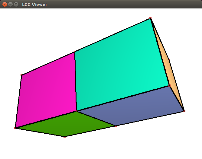
A linear cell complex can be visualized by calling the CGAL::draw<LCC>() function as shown in the following example. This function opens a new window showing the given linear cell complex. A call to this function is blocking, that is the program continues as soon as the user closes the window.
File Linear_cell_complex/draw_linear_cell_complex.cpp
This function requires CGAL_Qt5, and is only available if the flag CGAL_USE_BASIC_VIEWER is defined at compile time.
This package was developed by Guillaume Damiand, with the help of Andreas Fabri, Sébastien Loriot and Laurent Rineau. Monique Teillaud and Bernd Gärtner contributed to the manual.
 1.8.13