This chapter describes the Cgal 2D streamline placement package. Basic definitions and notions are given in Section 53.1. Section 53.2 gives a description of the integration process. Section 53.3 provides a brief description of the algorithm. Section 53.4 presents the implementation of the package, and Section 53.5 details two example placements.
53.1 Definitions
In physics, a field is an assignment of a quantity to every
point in space. For example, a gravitational field assigns a
gravitational potential to each point in space.
Vector and direction fields are commonly used for modeling physical
phenomena, where a direction and magnitude, namely a vector is assigned to
each point inside a domain (such as the magnitude and direction of the
force at each point in a magnetic field).
Streamlines are important tools for visualizing flow fields. A
streamline is a curve everywhere tangent to the field. In practice,
a streamline is often represented as a polyline (series of points)
iteratively elongated by bidirectional numerical integration started
from a seed point, until it comes close to another streamline
(according to a specified distance called the separating distance), hits the domain boundary, reaches a critical point or
generates a closed path.
A valid placement of streamlines consists of saturating the domain with a set of tangential streamlines in accordance with a specified density, determined by the separating distance between the streamlines.
53.2 Fundamental Notions
A streamline can be considered as the path traced by an imaginary massless particle dropped into a steady fluid flow described by the field. The construction of this path consists in the solving an ordinary differential equation for successive time intervals. In this way, we obtain a series of points pk, 0<k<n which allow visualizing the streamline. The differential equation is defined as follows :
| = v(p(t)), p(0) = p0 |
| p(t + Δt) = p(t) + ∫tt+Δt v(p(t)) dt |
53.2.1 Euler Integrator
This algorithm approximates the point computation by this formula
| pk+1 = pk + hv(pk) |
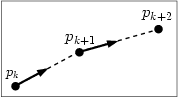
53.2.2 Second Order Runge-Kutta Integrator
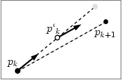
This method introduces an intermediate point p'k between pk and pk+1 to increase the precision of the computation (see Figure 53.3), where:
|
See [PTVF02] for further details about numerical integration.
53.3 Farthest Point Seeding Strategy
The algorithm implemented in this package [MAD05]
consists of placing one streamline at a time by numerical integration
starting farthest away from all previously placed
streamlines.
The input of our algorithm is given by (i) a flow field, (ii) a
density specified either globally, by the inverse of the
ideal spacing distance, or locally by a density field, and (iii) a
saturation ratio over the desired spacing required to trigger
the seeding of a new streamline.
The input flow field is given by a discrete set of vectors or
directions sampled within a domain, associated with an interpolation
scheme (e.g. bilinear interpolation over a regular grid, or
natural neighbor interpolation over an irregular point set to allow
for an evaluation at each point coordinate within the domain).
The output is a streamline placement, represented as a list
of streamlines. The core idea of our algorithm consists of placing
one streamline at a time by numerical integration seeded at the
farthest point from all previously placed streamlines.
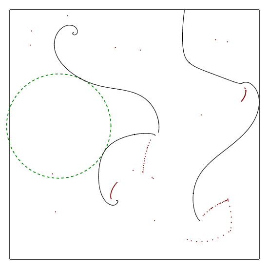
The streamlines are approximated by polylines, whose points are
inserted to a 2D Delaunay
triangulation (see figure 53). The empty circumscribed
circles of the Delaunay triangles provide us with a good approximation
of the cavities in the domain.
After each streamline integration, all incident triangles whose
circumcircle diameter is larger (within the saturation ratio) than the
desired spacing distance are pushed to a priority queue sorted by the
triangle circumcircle diameter. To start each new streamline
integration, the triangle with largest circumcircle diameter (and
hence the biggest cavity) is popped out of the queue. We first test if
it is still a valid triangle of the triangulation, since it could have
been destroyed by a streamline previously added to the
triangulation. If it is not, we pop another triangle out of the
queue. If it is, we use the center of its circumcircle as seed point
to integrate a new streamline.
Our algorithm terminates when the priority queue is empty. The size of the biggest cavity being monotonically decreasing, our algorithm guarantees the domain saturation.
53.4 Implementation
Streamlines are represented as polylines, and are obtained by
iterative integration from the seed point. A polyline is represented as a range of points. The computation is
processed via a list of Delaunay triangulation vertices.
To implement the triangular grid, the Cgal Delaunay_triangulation_2 class is used. The priority queue used to store candidate seed points is taken from the Standard Template Library [Sil97].
53.5 Examples
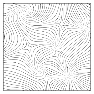
The first example illustrates the generation of a 2D streamline placement from a vector field defined on a regular grid.
File: examples/Stream_lines_2/stl_regular_field.cpp
#include <CGAL/Cartesian.h>
#include <CGAL/Filtered_kernel.h>
#include <CGAL/Stream_lines_2.h>
#include <CGAL/Runge_kutta_integrator_2.h>
#include <CGAL/Regular_grid_2.h>
#include <CGAL/Triangular_field_2.h>

#include <iostream>
#include <fstream>

typedef double coord_type;
typedef CGAL::Cartesian<coord_type> K1;
typedef CGAL::Filtered_kernel<K1> K;
typedef CGAL::Regular_grid_2<K> Field;
typedef CGAL::Runge_kutta_integrator_2<Field> Runge_kutta_integrator;
typedef CGAL::Stream_lines_2<Field, Runge_kutta_integrator> Strl;
typedef Strl::Point_iterator_2 Point_iterator;
typedef Strl::Stream_line_iterator_2 Strl_iterator;
typedef Strl::Point_2 Point_2;
typedef Strl::Vector_2 Vector_2;

int main()
{
  Runge_kutta_integrator runge_kutta_integrator;

  /*data.vec.cin is an ASCII file containing the vector field values*/
  std::ifstream infile("data/vnoise.vec.cin", std::ios::in);
  double iXSize, iYSize;
  unsigned int x_samples, y_samples;
  iXSize = iYSize = 512;
  infile >> x_samples;
  infile >> y_samples;
  Field regular_grid_2(x_samples, y_samples, iXSize, iYSize);
  /*fill the grid with the appropreate values*/
  for (unsigned int i=0;i<x_samples;i++)
    for (unsigned int j=0;j<y_samples;j++)
      {
        double xval, yval;
        infile >> xval;
        infile >> yval;
        regular_grid_2.set_field(i, j, Vector_2(xval, yval));
      }
  infile.close();

  /* the placement of streamlines */
  std::cout << "processing...\n";
  double dSep = 3.5;
  double dRat = 1.6;
  Strl Stream_lines(regular_grid_2, runge_kutta_integrator,dSep,dRat);
  std::cout << "placement generated\n";

  /*writing streamlines to streamlines_on_regular_grid_1.stl */
  std::ofstream fw("streamlines_on_regular_grid_1.stl",std::ios::out);
  fw << Stream_lines.number_of_lines() << "\n";
  for(Strl_iterator sit = Stream_lines.begin(); sit != Stream_lines.end(); sit++)
    {
      fw << "\n";
      for(Point_iterator pit = sit->first; pit != sit->second; pit++){
        Point_2 p = *pit;
        fw << p.x() << " " << p.y() << "\n";
      }
    }

  fw.close();

}
The second example depicts the generation of a streamline placement from a vector
field defined on a triangular grid.
File: examples/Stream_lines_2/stl_triangular_field.cpp
#include <CGAL/Cartesian.h>
#include <CGAL/Filtered_kernel.h>
#include <CGAL/Stream_lines_2.h>
#include <CGAL/Runge_kutta_integrator_2.h>
#include <CGAL/Triangular_field_2.h>

#include <iostream>
#include <fstream>

typedef double                                                      coord_type;
typedef CGAL::Cartesian<coord_type>                                 K1;
typedef CGAL::Filtered_kernel<K1> K;
typedef K::Point_2                                                  Point;
typedef K::Vector_2                                                 Vector;
typedef CGAL::Triangular_field_2<K>                                 Field;
typedef CGAL::Runge_kutta_integrator_2<Field>                       Runge_kutta_integrator;
typedef CGAL::Stream_lines_2<Field, Runge_kutta_integrator>         Strl;
typedef Strl::Stream_line_iterator_2                                 stl_iterator;

int main()
{
  Runge_kutta_integrator runge_kutta_integrator(1);

  /*datap.tri.cin and datav.tri.cin are ascii files where are stored the vector velues*/
  std::ifstream inp("data/datap.tri.cin");
  std::ifstream inv("data/datav.tri.cin");
  std::istream_iterator<Point> beginp(inp);
  std::istream_iterator<Vector> beginv(inv);
  std::istream_iterator<Point> endp;

  Field triangular_field(beginp, endp, beginv);

  /* the placement of streamlines */
  std::cout << "processing...\n";
  double dSep = 30.0;
  double dRat = 1.6;
  Strl Stream_lines(triangular_field, runge_kutta_integrator,dSep,dRat);
  std::cout << "placement generated\n";

  /*writing streamlines to streamlines.stl */
  std::cout << "streamlines.stl\n";
  std::ofstream fw("streamlines.stl",std::ios::out);
  Stream_lines.print_stream_lines(fw);
}