

|
CGAL 4.10 - 2D Envelopes
|
|
CGAL 4.10 - 2D Envelopes
|
A continuous curve \( C\) in \( {\mathbb R}^2\) is called \( x\)-monotone, if every vertical line intersects it at a single point at most. For example, the circle \( x^2 + y^2 = 1\) is not \( xy\)-monotone as the vertical line \( x = 0\) intersects it at \( (0, -1)\) and at \( (0, 1)\); however, it is possible to split the circle into an upper part and a lower part, such that both of these parts are \( x\)-monotone. We consider vertical segments as weakly \( x\)-monotone, to properly handle inputs that contain such vertical curves.
An \( x\)-monotone curve can be represented as a univariate function \( y = C(x)\), defined over some continuous range \( R_C \subseteq {\mathbb R}\). Given a set \( {\cal C} = \{ C_1, C_2, \ldots, C_n \}\) of \( x\)-monotone curves, their lower envelope is defined as the point-wise minimum of all curves. Namely, the lower envelope of the set \( {\cal C}\) can be defined as the following function:
\begin{eqnarray*} {\cal L}_{{\cal C}} (x) = \min_{1 \leq k \leq n}{\overline{C}_k (x)} \ , \end{eqnarray*}
where we define \(\overline{C}_k(x) = C_k(x)\) for \(x \in R_{C_k}\), and \(\overline{C}_k(x) = \infty\) otherwise.
Similarly, the upper envelope of \({\cal C}\) is the point-wise maximum of the \(x\)-monotone curves in the set:
\begin{eqnarray*} {\cal U}_{{\cal C}} (x) = \max_{1 \leq k \leq n}{\underline{C}_k (x)} \ , \end{eqnarray*}
where in this case \( \underline{C}_k(x) = -\infty\) for \( x \not\in R_{C_k}\).
Given a set of \( x\)-monotone curves \( {\cal C}\), the minimization diagram of \( {\cal C}\) is a subdivision of the \( x\)-axis into cells, such that the identity of the curves that induce the lower envelope over a specific cell of the subdivision (an edge or a vertex) is the same. In non-degenerate situations, an edge - which represents a continuous interval on the \( x\)-axis - is induced by a single curve (or by no curves at all, if there are no \( x\)-monotone curves defined over the interval), and a vertex is induced by a single curve and corresponds to one of its endpoints, or by two curves and corresponds to their intersection point. The maximization diagram is symmetrically defined for upper envelopes. In the rest of this chapter, we refer to both these diagrams as envelope diagrams.
Lower and upper envelopes can be efficiently computed using a divide-and-conquer approach. First, note that the envelope diagram for a single \( x\)-monotone curve \( C_k\) is trivial to compute: we project the boundary of its range of definition \( R_{C_k}\) onto the \( x\)-axis and label the features it induces accordingly. Given a set \( {\cal D}\) of (non necessarily \( x\)-monotone) curves in \( {\mathbb R}^2\), we subdivide each curve into a finite number of weakly \( x\)-monotone curves, and obtain the set \( {\cal C}\). Then, we split the set into two disjoint subsets \( {\cal C}_1\) and \( {\cal C}_2\), and we compute their envelope diagrams recursively. Finally, we merge the diagrams in linear time by traversing both diagrams in parallel.
The package basically contains two sets of free functions: lower_envelope_x_monotone_2(begin, end, diag) (similarly upper_envelope_x_monotone_2()) construct the envelope diagram for a given range of \( x\)-monotone curves, while lower_envelope_2(begin, end, diag) (similarly upper_envelope_2()) construct the envelope diagram for a range of arbitrary (not necessarily \( x\)-monotone) curves. In this section we explain more on the structure of the envelope diagram these functions output.
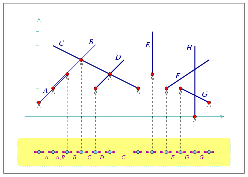
envelope_segments.cpp. The minimization diagram is shown at the bottom, where each diagram vertex points to the point associated with it, and the labels of the segment that induce a diagram edge are displayed below this edge. Note that there exists one edge that represents an overlap (i.e., there are two segments that induce it), and there are also a few edges that represent empty intervals. A minimization diagram or a maximization diagram is represented by a model of the concept EnvelopeDiagram_1. This concept defines the structure of the subdivision of the \( x\)-axis into 0-dimensional cells called vertices, and 1-dimensional cells called edges. The important property of this subdivision is that the identity of the curves that induce the lower envelope (or the upper envelope) over each cell is fixed.
Figure 36.2 shows the lower envelope of a set of eight line segments, and sketches the structure of their minimization diagram. Each diagram vertex \( v\) is associated with a point \( p_v\) on the envelope, which corresponds to either a curve endpoint or to an intersection point of two (or more) curves. The vertex is therefore associated with a set of \( x\)-monotone curves that induce the envelope over \( p_v\). Each vertex is incident to two edges, one lying to its left and the other to its right.
An edge in the envelope diagram represents a continuous portion of the \( x\)-axis, and is associated with a set of \( x\)-monotone curves that induce the envelope over this interval. Note that this set may be empty if no \( x\)-monotone curves are defined over this interval. In degenerate situations where curves overlap, there may be more than a single curve that induces the envelope over the interval the edge represents. An envelop diagram of a set of curves either consists of a single unbounded edge (in case the curve set is empty or if the envelope contains a single unbounded curve that is below or above all other curves), or at least one vertex and two unbounded edges, while each additional vertex comes along with an additional edge. It is possible to directly access the leftmost edge, representing the unbounded interval that starts at \( -\infty\), and the rightmost edge, representing the unbounded interval that ends at \( \infty\). (In the example depicted in Figure 36.2 we have only bounded curves, so the leftmost and rightmost edges represent empty intervals. This is not the case when we deal, for example, with envelopes of sets of lines.)
Any model of the EnvelopeDiagram_1 concept must define a geometric traits class, which in turn defines the Point_2 and X_monotone_curve_2 types defined with the diagram features. The geometric traits class must be a model of the ArrangementXMonotoneTraits_2 concept in case we construct envelopes of \( x\)-monotone curves. If we are interested in handling arbitrary (not necessarily \( x\)-monotone) curves, the traits class must be a model of the ArrangementTraits_2 concept. This concepts refined the ArrangementXMonotoneTraits_2 concept; a traits class that models this concepts must also defines a Curve_2 type, representing an arbitrary planar curve, and provide a functor for subdividing such curves into \( x\)-monotone subcurves.
The following example demonstrates how to compute and traverse the minimization diagram of line segments, as illustrated in Figure 36.2. We use the curve-data traits instantiated by the Arr_segment_traits_2 class, in order to attach a label (a char in this case) to each input segment. We use these labels when we print the minimization diagram.
File Envelope_2/envelope_segments.cpp
The next example computes the convex hull of a set of input points by constructing envelopes of unbounded curves, in our case lines that are dual to the input points. Here use the Arr_linear_traits_2 class to compute the lower envelope of the set of dual lines. We read a set of points \( {\cal P} = p_1, \ldots, p_n\) from an input file, and construct the corresponding dual lines \( {\cal P}^{*} = p^{*}_1, \ldots, p^{*}_n\), where the line \( p^{*}\) dual to a point \( p = (p_x, p_y)\) is given by \( y = p_x x - p_y\). We then compute the convex hull of the point-set \( {\cal P}\), using the fact that the lines that form the lower envelope of \( {\cal P}^{*}\) are dual to the points along the upper part of \( {\cal P}\)'s convex hull, and the lines that form the upper envelope of \( {\cal P}^{*}\) are dual to the points along the lower part of the convex hull; see, e.g., [1], Section 11.4 for more details. Note that the leftmost edge of the minimization diagram is associated with the same line as the rightmost edge of the maximization diagram, and vice-verse. We can therefore skip the rightmost edges of both diagrams.
File Envelope_2/convex_hull.cpp
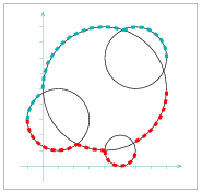
We conclude by an example of envelopes of non-linear curves. We use the Arr_circle_segment_traits_2 class to construct the lower and the upper envelopes of a set of four circles, as depicted in Figure 36.3. Note that unlike the two previous examples, here our curves are not \( x\)-monotone, so we use the functions that compute envelopes of arbitrary curves.
File Envelope_2/envelope_circles.cpp
 1.8.4
1.8.4