|
CGAL 4.7 - Surface Reconstruction from Point Sets
|
|
CGAL 4.7 - Surface Reconstruction from Point Sets
|
This CGAL component implements a surface reconstruction method which takes as input point sets with oriented normals and computes an implicit function. We assume that the input points contain no outliers and little noise. The output surface mesh is generated by extracting an isosurface of this function with the CGAL Surface Mesh Generator [4] or potentially with any other surface contouring algorithm.
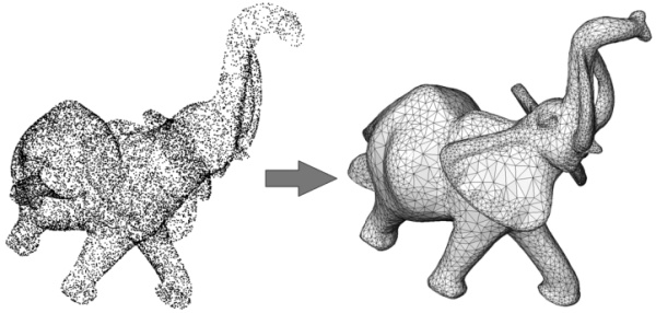
More specifically, the core surface reconstruction algorithm consists of computing an implicit function which is an approximate indicator function of the inferred solid (Poisson Surface Reconstruction - referred to as Poisson). Poisson is a two steps process: it requires solving for the implicit function before function evaluation.
Surface reconstruction from point sets is often a sequential process with the following steps: 1) Scanning and scan alignment produce a set of points or points with normals; 2) Outlier removal; 3) Simplification to reduce the number of input points; 4) Smoothing to reduce noise in the input data; 5) Normal estimation and orientation when the normals are not already provided by the acquisition device; and 6) Surface reconstruction.
CGAL provides algorithms for all steps listed above except alignment.
Chapter Point Set Processing describes algorithms to pre-process the point set before reconstruction with functions devoted to the simplification, outlier removal, smoothing, normal estimation and normal orientation.
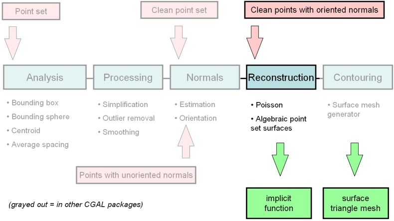
Given a set of 3D points with oriented normals (denoted oriented points in the sequel) sampled on the boundary of a 3D solid, the Poisson Surface Reconstruction method [2] solves for an approximate indicator function of the inferred solid, whose gradient best matches the input normals. The output scalar function, represented in an adaptive octree, is then iso-contoured using an adaptive marching cubes.
CGAL implements a variant of this algorithm which solves for a piecewise linear function on a 3D Delaunay triangulation instead of an adaptive octree. The algorithm takes as input a set of 3D oriented points. It builds a 3D Delaunay triangulation from these points and refines it by Delaunay refinement so as to remove all badly shaped (non isotropic) tetrahedra and to tessellate a loose bounding box of the input oriented points. The normal of each Steiner point added during refinement is set to zero. It then solves for a scalar indicator function \( f\) represented as a piecewise linear function over the refined triangulation. More specifically, it solves for the Poisson equation \( \Delta f = div(\mathbf{n})\) at each vertex of the triangulation using a sparse linear solver. Eventually, the CGAL surface mesh generator extracts an isosurface with function value set by default to be the median value of \( f\) at all input points.
The class template declaration is template<class Gt> class Poisson_reconstruction_function wher Gt is a geometric traits class.
For details see: Poisson_reconstruction_function<GeomTraits>
The following example reads a point set, creates a Poisson implicit function and reconstructs a surface.
File Surface_reconstruction_points_3/poisson_reconstruction_example.cpp
The computed implicit functions can be iso-contoured to reconstruct a surface by using the CGAL surface mesh generator [4] [1] :
The parameter Tag affects the behavior of make_surface_mesh():
Manifold_tag: the output mesh is guaranteed to be a manifold surface without boundary.Manifold_with_boundary_tag: the output mesh is guaranteed to be manifold and may have boundaries.Non_manifold_tag: the output mesh has no guarantee and hence is outputted as a polygon soup.The surface reconstructed by make_surface_mesh() is required to be a model of the concept SurfaceMeshComplex_2InTriangulation_3, a data structure devised to represent a two dimensional complex embedded into a three dimensional triangulation.
SurfaceMeshComplex_2InTriangulation_3 defines the methods to traverse the reconstructed surface, and e.g. convert it to a triangle soup.
Other CGAL components provide functions to write the reconstructed surface mesh to the Object File Format (OFF) [3] and to convert it to a polyhedron (when it is manifold):
See poisson_reconstruction_example.cpp example above.
The surface reconstruction problem being inherently ill-posed, the proposed algorithm does not pretend to reconstruct all kinds of surfaces with arbitrary sampling conditions. This section provides the user with some hints about the ideal sampling and contouring conditions, and depicts some failure cases when these conditions are not matched.
The user must keep in mind that the Poisson surface reconstruction algorithm comprises two phases (computing the implicit function from the input point set and contouring an iso-surface of this function). Both require some care in terms of sampling conditions and parameter tuning.
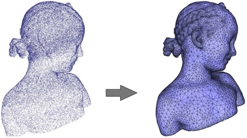
Ideally the current implementation of the Poisson surface reconstruction method expects a dense 3D oriented point set (typically matching the epsilon-sampling condition [1]) and sampled over a closed, smooth surface. Oriented herein means that all 3D points must come with consistently oriented normals to the inferred surface. Figure 52.3 and Figure 52.4 illustrate cases where these ideal conditions are met.
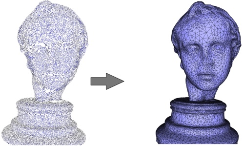
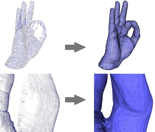
The algorithm is fairly robust to anisotropic sampling and to noise. It is also robust to missing data through filling the corresponding holes as the algorithm is designed to reconstruct the indicator function of an inferred solid (see Figure 52.5).
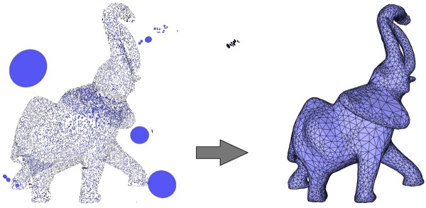
The algorithm is in general not robust to outliers, although a few outliers do not always create a failure, see Figure 52.6.
The algorithm works well even when the inferred surface is composed of several connected components, provided that both all normals are properly estimated and oriented (the current CGAL normal orienter algorithm may fail in some cases, see mst_orient_normals()), and that the final contouring algorithm is properly seeded for each component. When the inferred surface is composed of several nested connected components care should be taken to orient the normals of each component in alternation (inward/outward) so that the final contouring stage picks a proper contouring value.
Our implementation of the Poisson surface reconstruction algorithm computes an implicit function represented as a piecewise linear function over the tetrahedra of a 3D Delaunay triangulation constructed from the input points then refined through Delaunay refinement. For this reason, any iso-surface is also piecewise linear and hence may contain sharp creases. As the contouring algorithm make_surface_mesh() expects a smooth implicit function these sharp creases may create spurious clusters of vertices in the final reconstructed surface mesh when setting a small mesh sizing or surface approximation error parameter (see Figure 52.7).
One way to avoid these spurious clusters consists of adjusting the mesh sizing and surface approximation parameters large enough compared to the average sampling density (obtained through compute_average_spacing()) so that the contouring algorithm perceives a smooth iso-surface. We recommend to use the following contouring parameters:
The conditions listed above are rather restrictive and in practice not all of them are met in the applications. We now illustrates the behavior of the algorithm when the conditions are not met in terms of sampling, wrongly oriented normals, noise and sharp creases.
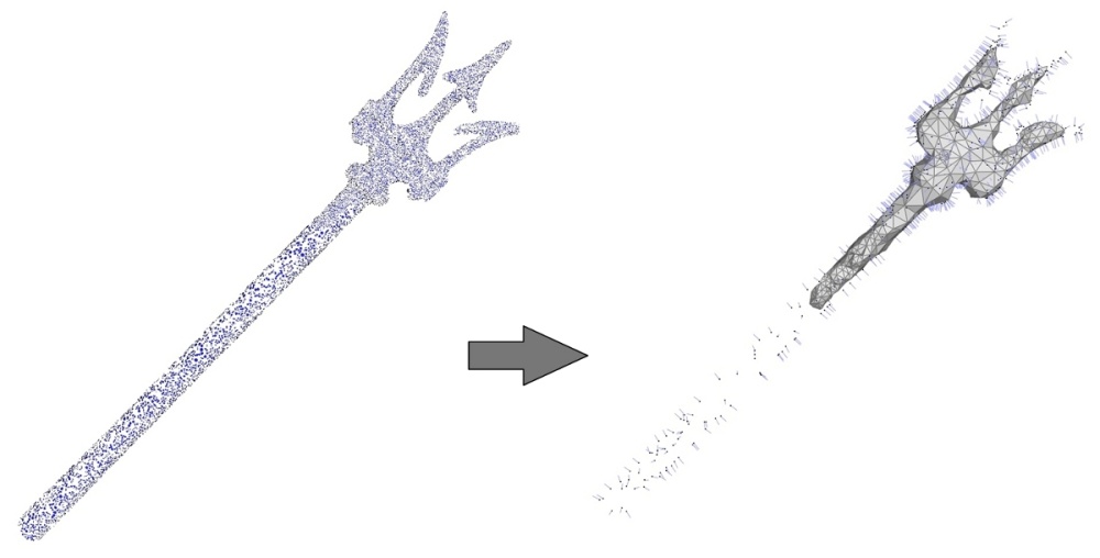
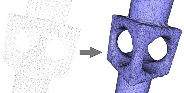
The reconstruction algorithm expects a sufficiently dense point set. Although there is no formal proof of correctness of the algorithm under certain density conditions due to its variational nature, our experiments show that the algorithm reconstructs well all thin features when the local spacing is at most one tenth of the local feature size (the distance to the medial axis, which captures altogether curvature, thickness and separation). When this condition is not met the reconstruction does not reconstruct the thin undersampled features (see Figure 52.8).
The reconstruction is devised to solve for an implicit function which is an approximate indicator function of an inferred solid. For this reason the contouring algorithm always extracts a closed surface mesh and hence is able to fill the small holes where data are missing due, e.g., to occlusions during acquisition (see Figure 52.9).
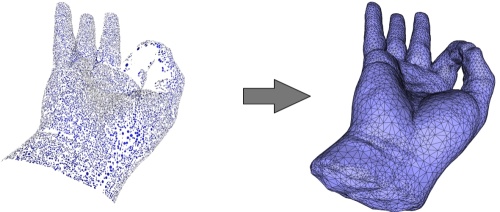
In case of large holes the algorithm still closes them all but the resulting piecewise linear implicit function may exhibit large triangle patches and sharp creases as the 3D Delaunay triangulation used for solving is very coarse where the holes are filled. This can be avoided by a two pass approach. The first pass for a subset of the points serves to get an approximation of the surface at the holes. This surface then serves to compute a smoother 3D Delaunay triangulation for the second pass with the full set of points.

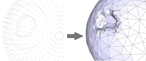
The Poisson surface reconstruction approaches solves for an implicit function whose gradient best matches a set of input normals. Because it solves this problem in the least squares sense, it is robust to few isolated wrongly oriented (flipped) normals. Nevertheless a cluster of wrongly oriented normals leads to an incorrect implicit function and hence to spurious geometric or even topological distortion (see Figure 52.11).
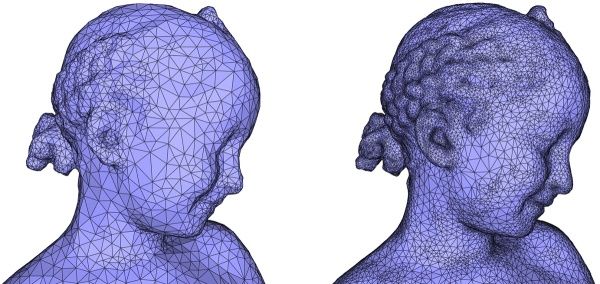
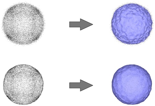
A large amount of noise inevitably impacts on the reconstruction (see Figure 52.12, top) and the current implementation does not provide any mean to trade data fitting for smoothness. Nevertheless if the signal-to-noise ratio is sufficiently high and/or the surface approximation and sizing parameters set for contouring the iso-surface is large with respect to the noise level the output surface mesh will appear smooth (not shown). If the user wants to produce a smooth and detailed output surface mesh, we recommend to apply smoothing through jet_smooth_point_set() (see Figure 52.12, bottom).
For a large number of outliers the failure cases (not shown) translate into spurious small connected components and massive distortion near the inferred surface. In this case the outliers must be removed through remove_outliers().
The current reconstruction algorithm is not able to recover the sharp creases and corners present in the inferred surface. This translates into smoothed sharp creases.
We provide some performance numbers for scanning data. We measure the Poisson implicit function computation time, the contouring time for a range of approximation distances, the memory occupancy as well as the influence of the point set simplification. The machine used is a PC running Windows 7 64 bits with an Intel CPU Core 2 Duo processor clocked at 2.81 GHz and with 8 GB of RAM. The software is compiled with Visual C++ 2010 (VC9) compiler with the 03 option which maximizes speed. All measurements were done using the Eigen library.
The point set chosen for benchmarking the Poisson implicit function is the Bimba con Nastrino point set (1.6 million points) depicted by Figure 52.14. We measure the Poisson implicit function computation (i.e., the call to Poisson_reconstruction_function::compute_implicit_function() denoted by Poisson solve hereafter) for this point set as well as for simplified versions obtained through random simplification. The following table provides Poisson solve computation times in seconds for an increasing number of points.
|
Number of points (x1000) | Poisson solve duration (in s) |
| 60 | 15 |
| 100 | 25 |
| 250 | 96 |
| 500 | 150 |
| 1,000 | 249 |
| 1,800 | 478 |
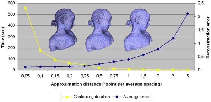
The point set chosen for benchmarking the contouring stage is the Bimba con Nastrino point set simplified to 100k points. We measure the contouring (i.e. the call to make_surface_mesh()) duration and the reconstruction error for a range of approximation distances. The reconstruction error is expressed as the average distance from input points to the reconstructed surface in mm (the Bimba con Nastrino statue is 324 mm tall).
| Approx. distance (*average spacing) | Contouring duration (in s) | Reconstruction error (mm) |
| 0.1 | 19.2 | 0.055 |
| 0.25 | 6.9 | 0.106 |
| 0.5 | 3.2 | 0.18 |
| 1 | 1.65 | 0.36 |
| 2 | 0.8 | 0.76 |
We measure the memory occupancy for the reconstruction of the full Bimba con Nastrino point set (1.8 millions points) as well as for simplified versions.
The Poisson implicit function computation has a memory peak when solving the Poisson linear system using the sparse linear solver.
| Number of points (x1000) | Memory occupancy (MBytes) |
| 60 | 180 |
| 100 | 270 |
| 250 | 790 |
| 500 | 1300 |
| 1,000 | 2200 |
| 1,800 | 3800 |
Due to the memory limitations described above, we recommend to simplify the point sets captured by laser scanners.
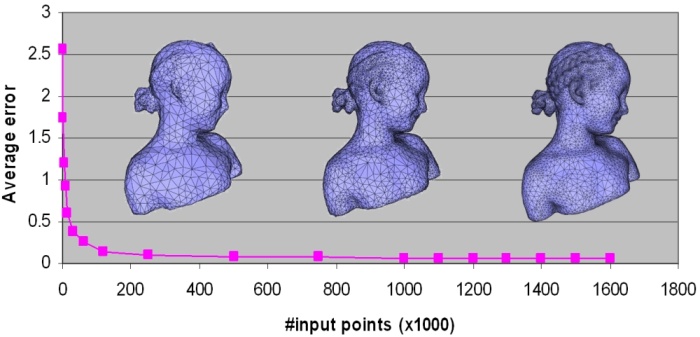
We measure the reconstruction error for the Bimba con Nastrino point set (1.6M points) as well as for simplified versions. All reconstructions use the recommended contouring parameter approximation distance = 0.25 * the input point set's average spacing. The reconstruction error is expressed as the average distance from input points to the reconstructed surface in mm (the Bimba con Nastrino statue is 324 mm tall).
| Number of points (x1000) | Reconstruction error (mm) |
| 60 | 0.27 |
| 120 | 0.15 |
| 250 | 0.11 |
| 500 | 0.079 |
| 1,000 | 0.066 |
| 1,500 | 0.061 |
| 1,600 | 0.06 |
The initial implementation was essentially done by Laurent Saboret, guided by Pierre Alliez and Ga"el Guennebaud. For later releases of the package Andreas Fabri worked on performance improvements, and Laurent Rineau added the two passes for dealing with holes.