|
CGAL 5.1.5 - Triangulated Surface Mesh Shortest Paths
|
|
CGAL 5.1.5 - Triangulated Surface Mesh Shortest Paths
|
This package provides an algorithm to compute geodesic shortest paths on a triangulated surface mesh.
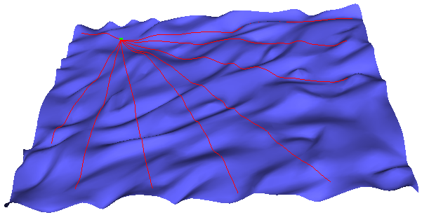
The motion planning of a robot across the surface of a 3-dimensional terrain is a typical application of the shortest path computation. Using a 2-dimensional approximation would fail to capture anything interesting about the terrain we are trying to cross, and would give a poor solution. The problem is often called the Discrete Geodesic Problem. Although the more general version of this problem, shortest paths in 3D in the presence of obstacles, is NP-Hard, when the motion is constrained to the 2D surface of an object it can be solved efficiently.
The algorithm implemented in this package builds a data structure to efficiently answer queries of the following form: Given a triangulated surface mesh \(\cal{M}\), a set of source points \(S\) on \(\cal{M}\), and a target point \(t\) also on \(\cal{M}\), find a shortest path \(\lambda\) between \(t\) and any element in \( S \), where \(\lambda\) is constrained to the surface of \(\cal{M}\).
The algorithm used is based on a paper by Xin and Wang [3], a fast and practical algorithm for exact computation of geodesic shortest paths. It is an extension of earlier results by Chen and Han [1] and Mitchell, Mount, and Papadimitriou [2] .
This package is related to the package Heat Method Reference. Both deal with geodesic distances. The geodesic shortest path package computes the exact shortest path between any two points on the surface. The heat method package computes for every vertex of a mesh an approximate distance to one or several source vertices.
The main class of this package is Surface_mesh_shortest_path. In the following we describe the typical workflow when using this class
The shortest paths are computed on a triangulated surface mesh, represented by a model of the FaceListGraph concept. There is no restriction on the genus, connectivity, or convexity of the input surface mesh.
For efficiency reason, index property maps for vertices, halfedges and faces are internally used. For each simplex type the property map must provide an index between 0 and the number of simplices. We recommend to use the class CGAL::Surface_mesh as model of FaceListGraph. If you use the class CGAL::Polyhedron_3, you should use it with the item class CGAL::Polyhedron_items_with_id_3, for which default property maps are provided. This item class associates to each simplex an index that provides a \(O(1)\) time access to the indices. Note that the initialization of the property maps requires a call to set_halfedgeds_items_id().
The access to the embedding of each vertex is done using a point vertex property map associating to each vertex a 3D point. Defaults are provided for CGAL classes.
If the traits class used holds some local state, it must also be passed to the class when constructing it (the default one provided does not).
The set of source points for shortest path queries can be populated one by one or using a range. A source point can be specified using either a vertex of the input surface mesh or a face of the input surface mesh with some barycentric coordinates. Given a point \(p\) that lies inside a triangle face \((A,B,C)\), its barycentric coordinates are a weight triple \((b_0,b_1,b_2)\) such that \(p = b_0\cdot~A + b_1\cdot~B + b_2\cdot~C\), and \(b_0 + b_1 + b_2 = 1\).
For convenience, a function Surface_mesh_shortest_path::locate() is provided to construct face locations from geometric inputs:
p living in 3D space, this function computes the point closest to p on the surface, and returns the face containing this point, as well as its barycentric coordinates;r living in 3D space, this function computes the intersection of the ray with the surface, and (if an intersection exists) returns the face containing this point, as well as its barycentric coordinates;Usage of this function is illustrated in the example Surface_mesh_shortest_path/shortest_path_with_locate.cpp.
A time consuming operation for shortest path queries consists in building an internal data structure used to make the queries. This data structure is called the sequence tree. It will be built automatically when the first shortest path query is done and will be reused for any subsequent query as long as the set of source points does not change. Each time the set of source points is changed the sequence tree needs to be rebuilt (if already built). Note that it can also be built manually by a call to Surface_mesh_shortest_path::build_sequence_tree().
As for specifying the source points, the target point for a shortest path query can be specified using either a vertex of the input surface mesh or a face of the input surface mesh and some barycentric coordinates.
There are three different kinds of query functions that can be called using the class Surface_mesh_shortest_path. Given a target point, all these functions compute the shortest path between that target point and the set of source points:
Surface_mesh_shortest_path::shortest_distance_to_source_points() provides the closest source point to the target point together with the length of the shortest path.Surface_mesh_shortest_path::shortest_path_points_to_source_points() provides all the intersection points of the shortest path with the edges and vertices of the input surface mesh (including the source and the target point). This function is useful for visualization purposes.Surface_mesh_shortest_path::shortest_path_sequence_to_source_points gives access to the complete sequence of simplices crossed by the shortest path using a visitor object model of the concept SurfaceMeshShortestPathVisitor.Some convenience functions are provided to compute:
CGAL::AABB_tree.In short, we recommend to use a CGAL kernel with exact predicates such as CGAL::Exact_predicates_inexact_constructions_kernel.
If you need the constructions to be exact (for the shortest path point computation for example), you should use a kernel with exact constructions. Although the algorithm uses square root operations, it will also work on geometry kernels which do not support them by first converting the kernel's number type to double, using the std::sqrt, and converting it back. Note that it would be preferable to use a kernel with directly supports square roots to get the most precision of the shortest path computations.
Using a kernel such as CGAL::Exact_predicates_exact_constructions_kernel_with_sqrt with this package will indeed provide the exact shortest paths, but it will be extremely slow. Indeed, in order to compute the distance along the surface, it is necessary to unfold sequences of faces, edge-to-edge, out into a common plane. The functor SurfaceMeshShortestPathTraits::Construct_triangle_3_to_triangle_2_projection provides an initial layout of the first face in a sequence, by rotating a given face into the xy-plane. SurfaceMeshShortestPathTraits::Construct_triangle_3_along_segment_2_flattening unfolds a triangle into the plane, using a specified segment as a base. Since this results in a chain of constructed triangles in the plane, the exact representation types used with this kernel (either CORE::Expr or leda_real) will process extremely slow, even on very simple inputs. This is because the exact representations will effectively add an \(O(n)\) factor to every computation.
The following example shows how to get the shortest path to every vertex from an arbitrary source point on a surface. The shortest path class needs to have an index associated to each vertex, halfedge and face, which is naturally given for the class Surface_mesh.
File Surface_mesh_shortest_path/shortest_paths.cpp
The following example shows how to get the shortest path to every vertex from an arbitrary source point on the surface. Note that this example uses the Polyhedron_items_with_id_3 item class. The shortest path class needs to have an index associated to each vertex, halfedge and face. Using this item class provide an efficient direct access to the required indices.
File Surface_mesh_shortest_path/shortest_paths_with_id.cpp
Although it is better to have an index built into each simplex, you can also use a surface mesh without internal indices by using external indices. The following example shows how to proceed in this case.
File Surface_mesh_shortest_path/shortest_paths_no_id.cpp
This example shows how to compute the sequence tree from multiple source points, using an iterator range of Surface_mesh_shortest_path::Face_location objects generated at random.
File Surface_mesh_shortest_path/shortest_paths_multiple_sources.cpp
This example shows how to implement a model of the SurfaceMeshShortestPathVisitor concept to get detailed information about the sequence of simplicies crossed by a shortest path.
File Surface_mesh_shortest_path/shortest_path_sequence.cpp
These benchmarks were run using randomly generated source and destination points over multiple trials. The measurements were executed using CGAL 4.5, under Cygwin 1.7.32, using the Gnu C++ compiler version 4.8.3 with options -O3 -DNDEBUG. The system used was a 64bit Intel Core i3 2.20GHz processor with 6GB of RAM
| Model | Number of Vertices | Average Construction Time (s) | Average Queries Per Second | Peak Memory Usage (MB) |
|---|---|---|---|---|
| ellipsoid.off | 162 | 0.00258805 | 1.21972e+06 | 0.39548 |
| anchor.off | 519 | 0.0580262 | 230461 | 3.88799 |
| rotor.off | 600 | 0.0386633 | 326175 | 3.10571 |
| spool.off | 649 | 0.0418305 | 299766 | 3.75773 |
| handle.off | 1165 | 0.0976167 | 227343 | 7.66706 |
| couplingdown.off | 1841 | 0.138467 | 246833 | 10.1731 |
| bones.off | 2154 | 0.0101125 | 1.31834e+06 | 0.865896 |
| mushroom.off | 2337 | 0.206034 | 202582 | 22.5804 |
| elephant.off | 2775 | 0.136177 | 313785 | 14.0987 |
| cow.off | 2904 | 0.259104 | 206515 | 17.4796 |
| knot1.off | 3200 | 0.279455 | 207084 | 25.314 |
| retinal.off | 3643 | 0.255788 | 247617 | 29.8031 |
| femur.off | 3897 | 0.25332 | 264825 | 21.4806 |
| knot2.off | 5760 | 0.295655 | 309593 | 22.5549 |
| bull.off | 6200 | 0.513506 | 209994 | 34.983 |
| fandisk.off | 6475 | 0.609507 | 198768 | 71.3617 |
| lion-head.off | 8356 | 1.23863 | 145810 | 86.6908 |
| turbine.off | 9210 | 2.23755 | 93079.5 | 172.072 |
| man.off | 17495 | 1.59015 | 187519 | 148.358 |
| Model | Number of Vertices | Average Construction Time (s) | Average Queries Per Second | Peak Memory Usage (MB) |
|---|---|---|---|---|
| ellipsoid.off | 162 | 0.00321017 | 911025 | 0.245674 |
| anchor.off | 519 | 0.03601 | 353062 | 3.19274 |
| rotor.off | 600 | 0.015864 | 805416 | 1.97554 |
| spool.off | 649 | 0.0165743 | 802701 | 2.09675 |
| handle.off | 1165 | 0.0294564 | 646057 | 4.62122 |
| couplingdown.off | 1841 | 0.126045 | 272465 | 7.80517 |
| bones.off | 2154 | 0.055434 | 536646 | 4.0203 |
| mushroom.off | 2337 | 0.139285 | 290425 | 11.462 |
| elephant.off | 2775 | 0.167269 | 285076 | 11.2743 |
| cow.off | 2904 | 0.15432 | 328549 | 13.0676 |
| knot1.off | 3200 | 0.114051 | 454640 | 16.1735 |
| retinal.off | 3643 | 0.233208 | 287869 | 18.6274 |
| femur.off | 3897 | 0.128097 | 457112 | 16.8295 |
| knot2.off | 5760 | 0.413548 | 260195 | 33.484 |
| bull.off | 6200 | 0.371713 | 297560 | 30.522 |
| fandisk.off | 6475 | 0.545929 | 223865 | 39.5607 |
| lion-head.off | 8356 | 0.70097 | 229449 | 59.6597 |
| turbine.off | 9210 | 1.35703 | 157301 | 90.7139 |
| man.off | 17495 | 1.75936 | 185194 | 122.541 |
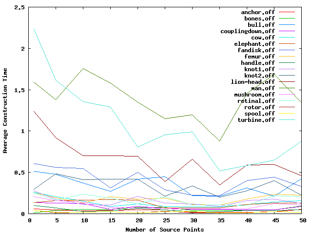
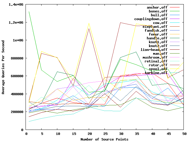
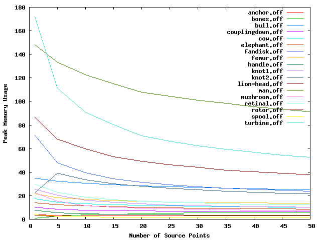
The following figures track the construction time, query time, and peak memory usage for the various test models as the number of source points increases. Notice that none of the values increases significantly as the number of source points increases. In fact, in most cases, the running time and memory go down. This is because a larger number of source points tends to result in a more flat sequence tree, which translates to reduced runtime and memory costs.
A geodesic curve is a locally shortest path on the surface of some manifold, that is, it cannot be made shorter by some local perturbations. On a surface mesh, this translates to a curve where, when the faces crossed by the curve are unfolded into the plane, the curve forms a straight line. Another way of describing it is that there is exactly \(\pi\) surface angle to both sides at every point along the curve (except possibly at the curve's endpoints).
A geodesic curve between two points is not necessarily a shortest path, but all shortest paths on surface meshes are formed by sequences of one or more geodesic paths, whose junction points are either vertices on the boundary of the mesh, or saddle vertices. We call such a curve on the surface of the mesh a potential shortest path between its two endpoints.
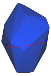
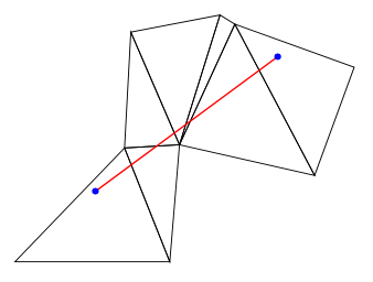
A visibility window (or visibility cone) is a pair of geodesic curves which share a common source point and enclose a locally flat region of the surface mesh. Locally flat means that between every pair of points inside the window, there is exactly one geodesic path between them which also stays inside the bounds of the window. Thus, operations, such as distance calculations, can be done with normal 2D Euclidean operations while inside the window. When a visibility window encounters a vertex (a non-flat part of the surface), a branch occurs, forming a sub-window to either side.
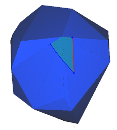
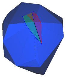
A saddle vertex on a surface mesh is a vertex \(v\) where the sum of surface angles of all faces incident at \(v\) is greater than \(2 \pi\), or, in simpler terms, one cannot flatten all the faces incident to \(v\) into the plane without overlap. Identifying and dealing with saddle vertices are important in shortest path algorithms because they form blind spots which cannot be reached by a single geodesic curve.
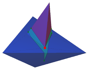
In order to deal with this, we must create a new set of child visibility windows which branch out around the saddle vertex. The paths through these child windows would first arrive at the saddle vertex, and then follow a new visibility window (forming a kind of poly-line on the surface). Note that similar behavior is required when we reach a boundary vertex of a non-closed surface mesh.
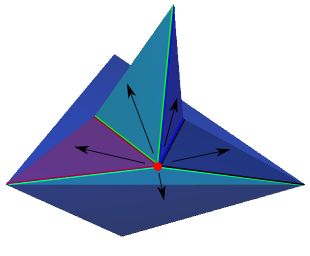
In order to compute shortest paths, we build a sequence tree (or cone tree) from each source point. The sequence tree describes the combinatoric structure of all potential shortest paths which originate from a single source point, by organizing them into a hierarchy of visibility windows.
Whenever a vertex of the surface mesh is encountered, a branch occurs in the sequence tree. If the vertex is a non-saddle vertex, then only two children are created, one for each edge incident to that vertex on the current face. If the vertex is a saddle vertex, in addition to the two children mentioned above, a special type of node, called a pseudo-source, is created which branches out from that vertex.
Once a sequence tree is built, the potential shortest paths from the source to every point inside a given visibility window can be computed. The sequence of faces along each branch of the tree are laid out edge to edge, into a common plane, such that the geodesic distance from any point on the surface to its nearest source point can be obtained using a single 2D Euclidean distance computation. Note that if the window belongs to a pseudo-source, the distance is measured from the target to the pseudo-source, and then the distance from the pseudo-source back to its parent is measured, and so on back to the original source.
The size of the sequence tree from any source point is theoretically infinite, however we only ever care about trees which are of depth at most N, where N is the number of faces in the surface mesh (since no shortest path can cross the same face twice). Even then, the size of this truncated sequence tree is potentially exponential in the size of the surface mesh, thus a simple breadth-first search is not feasible. Rather, we apply techniques to eliminate entire branches which are provably unable to contain shortest paths from the source point(s). The techniques used are given in greater detail in a paper by Xin and Wang [3], which itself expands an earlier work by Chen and Han [1] and Mitchell, Mount, and Papadimitriou [2] .
Handling multiple source points is simply a matter of constructing multiple sequence trees concurrently, using a method similar to the multi-source Dijsktra's algorithm.
Continuous Dijkstra is simply the application of the graph-search algorithm to a non-discrete setting. As we build the search tree, newly created nodes are tagged with a distance metric, and inserted into a priority queue, such that the shortest distance nodes are always first.
This observation by Chen and Han states that out of all the branches that occur at any given vertex of the surface mesh, only a limited number have more than one child which can define shortest paths. This is accomplished by maintaining, for each vertex, all nodes of the sequence tree which can contain that vertex inside their visibility window.
This method alone can decrease the running time for construction of the sequence tree construction to polynomial time.
An additional distance filter proposed by Xin and Wang helps prune the search tree even further by comparing the current node's distance to the closest distance so far of the three vertices on the current face. Details on this method can be found in their paper [3].
In order to locate the shortest path from a target point to a source point, we must select the correct visibility window. A simple method is to keep track for each face \(f\) of all windows which cross \(f\). In practice, at most a constant number of windows will cross any given face, so for simplicity this is the method we employ. An alternative is to construct a Voronoi-like structure on each face, where each cell represents a visibility window. We did not attempt this method, however it would seem likely that it would be of no computational benefit.
In this section we give a brief outline of the pseudo-code for this algorithm. More details can be found in [1] and [3].
--
-- Global Values
--
G : FaceGraph(V,E,F)
  -- V - the set of vertices
  -- E - the set of edges
  -- F - the set of planar faces

Q : PriorityQueue
  -- A priority queue ordered using the metric given by Xin and Wang

--
-- Types
--
type VisbilityWindow:
  f : a face of F, the current face of this window, we say this window 'crosses' face f
  s : a point on the surface of F, the source point of this window
  d :  the 'base distance' to s, only non-zero if s is a pseudo-source
  l : the left-side bounding ray of this window, with its origin at s
  r : the right-side bounding ray of this window, with its origin at s
  p : its parent VisibilityWindow

--
-- Methods
--
method XinWangDistanceFilter:
  Input:
    w : a VisibilityWindow
  Output:
    filter : true if w passes the distance filtering metric given by Xin and Wang, false otherwise

method PropagateWindow:
  Input:
    w : a visibility window
    e : an edge on face w.f
  Output:
    w' : A new visibility window on the face opposite w.f across edge e
  Begin:
    Let f' be the face on the opposite side of e as w.f
    Lay out face f' along e, such that it shares a common plane with w.f
    Create a new VisibilityWindow w', with
    - w its parent
    - the same source point and base distance as w
    - its boundary rays clipped to the sub-segment of e covered by w
    return w'

method CreateFaceWindow:
  Input:
    f : a face of F
    v : a vertex of f
    w : a VisibilityWindow which intersects f and contains v
  Output:
    w' : a new VisibilityWindow, with
    -- w its parent
    -- its source point s = v
    -- its two bounding rays along the edges incident to v
    -- face f as its crossed face
    -- its base distance being the distance of window w to v

method CreatePseudoSource:
  Input:
    w : the parent window
    v : a saddle vertex of V
  Begin:
    For each face f incident to v:
      w' = CreateFaceWindow(f, v, w)
      Q.insert(w')

method TreeDepth:
  Input:
    w : a VisibilityWindow in some sequence tree T
  Output:
    The depth of node w in its current sequence tree (this would typically be cached in w itself)

method ShortestPathTree:
  Input:
    s[1..n] : a set of source points on the surface of G.
              For simplicity (and without loss of generality),
              we will assume they are all vertices of G.
  Output:
    T[1..n] : a set of sequence trees for the source points
  Declare:
    O : a map of (f,v) => VisibilityWindow, which gives the 'vertex occupier' for (f,v),
        that is the window which crosses face f and whose source is nearest to vertex v
    S : a map of v => VisibilityWindow, which gives the window whose source is nearest
        to v. Note that this is a strict subset of O
  Begin:
    for i in 1..n:
      Let r[i] be the root of T[i], with distance 0 to s[i]
      CreatePseudoSource( r[i], s[i] )
    While Q is not empty:
      w = Q.take()
      if XinWangDistanceFilter(w) and TreeDepth(w) <= |F|:
        if w contains a vertex v of w.f:
          if w is closer to v than O[w.f,v]:
            O[w.f,v] = w
            if v is a boundary vertex or a saddle vertex, and w is closer to v than S[v]:
              S[v] = w
              CreatePseudoSource(w, v, w.dist(v))
            let {e_0, e_1} be the edges of f incident to v
            for i in [0,1]:
              w' = PropagateWindow(w, e_i)
              Q.insert(w')
          else:
            let e_n be the edge 'closer' to window w
            w' = PropagateWindow(w, e_n)
            Q.insert(w')
        else:
          let e_o be the only edge crossed by window w
          w' = PropagateWindow(w, e_o)
          Q.insert(w')
    return T[1..n]
To perform shortest path distance queries to each vertex, we can simply use the results stored in S after the completion of ShortestPathTree, as it contains a map from each vertex to the VisibilityWindow which has the shortest path to that vertex. Performing shortest path computations to any arbitrary face location is slightly more complex. As eluded to above, after completion of the algorithm, we traverse each of the sequence trees, and for each face f we store all the VisibilityWindows which cross f in a look-up structure. Then, to find the shortest path to a point on the surface of face f, we look up that pre-stored set of VisibilityWindows associated with it, and among those windows we select the one which contains the query point and has the shortest path back to the origin. Though it may seem slow since it involves a linear search but it is efficient in practice since the number of faces crossing any single face is typically limited (this is due to the additional filtering method given by Xin and Wang [3].
The actual surface paths can be reconstructed by backtracking from the VisibilityWindow, through its parents in the tree up to the root, and keeping track of each face that was crossed.
This package is the result of the work of Stephen Kiazyk during the 2014 season of the Google Summer of Code. He has been mentored by Sébastien Loriot and Éric Colin de Verdière who also contributed to the documentation and the API definition.