

|
CGAL 5.1 - Optimal Transportation Curve Reconstruction
|
|
CGAL 5.1 - Optimal Transportation Curve Reconstruction
|
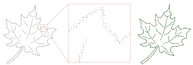
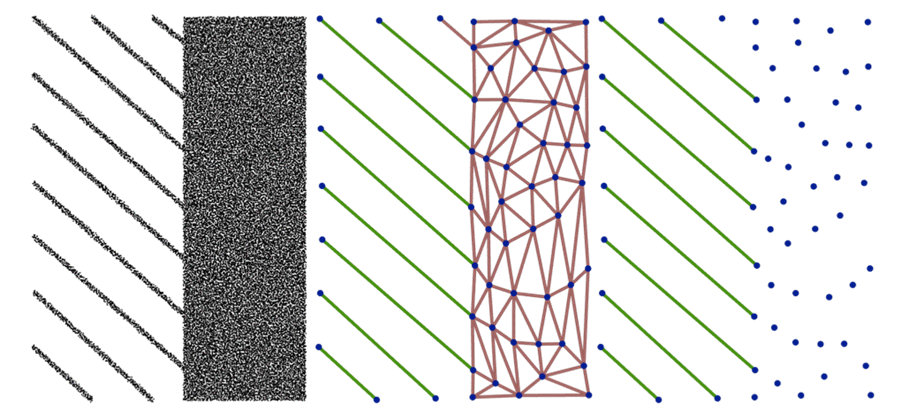
This package implements a method to reconstruct and simplify 2D point sets [1]. The input is a set of 2D points with mass attributes, possibly hampered by noise and outliers. The output is a set of line segments and isolated points which approximate the input points, as illustrated in Figure 64.1. The mass attribute relates to the importance given to each point for approximation.
Internally, the algorithm constructs an initial 2D Delaunay triangulation from all the input points, then simplifies the triangulation so that a subset of the edges and vertices of the triangulation approximate well the input points. Approximate herein refers to a robust distance based on optimal transportation (see section How Does It Work? for more details). The triangulation is simplified using a combination of half edge collapse, edge flips and vertex relocation operators. The triangulation remains valid during simplification, i.e., with neither overlaps nor fold-overs.
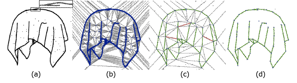
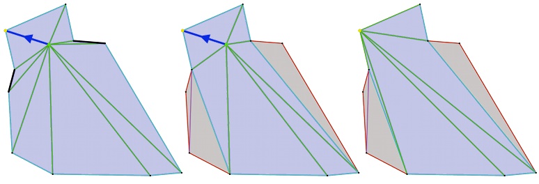
The output of the reconstruction algorithm is a subset of edges and vertices of the triangulation. Figure 64.2 depicts an example where the output is composed of green edges and one isolated vertex. The green edges are considered relevant as they approximate well many of the input points. The edges depicted in grey, referred to as ghost edges and discarded, approximate none of the input points. The edges depicted in red, referred to as irrelevant and also discarded, approximate some of the input points but not enough to be considered relevant.
The following example first generates a set of input points on a square. The points, with no mass attribute, are then passed to the Optimal_transportation_reconstruction_2 object. After initialization, 100 iterations of the reconstruction process are performed.
File Optimal_transportation_reconstruction_2/otr2_simplest_example.cpp
There is no direct relationship between the target number of edges for the output reconstruction and a notion of approximation error. The simplification algorithm can thus be stopped via a maximum tolerance error homogeneous to a distance. More specifically, the tolerance error is specified as the maximum square root of transport cost per unit of mass, which is homogeneous to a distance.
Note that the tolerance is given in the sense of the Wasserstein distance (see Wasserstein Distance). It is not a Hausdorff tolerance: it does not mean that the distance between the input samples and the output polyline is guaranteed to be less than tolerance. It means that the square root of transport cost per mass (homogeneous to a distance) is at most tolerance.
File Optimal_transportation_reconstruction_2/otr2_simplest_example_with_tolerance.cpp
The output of the reconstruction can be obtained in two ways: either as a sequence of 2D points and segments, or as an indexed format where the connectivity of the segments is encoded, hence the terms vertices and edges. The indexed format records a list of points, then pairs of point indices in the said list for the edges, and point indices for the isolated vertices.
File Optimal_transportation_reconstruction_2/otr2_list_output_example.cpp
File Optimal_transportation_reconstruction_2/otr2_indexed_output_example.cpp
The following example first reads a set of input points and masses from an ASCII file. Using two property maps, the points and their initial mass are passed to the Optimal_transportation_reconstruction_2 object. After initialization 100 iterations of the reconstruction process are performed, then the segments and isolated points of the reconstructed shape are extracted and printed to the console.
File Optimal_transportation_reconstruction_2/otr2_mass_example.cpp
The only class exposed to the user is the Optimal_transportation_reconstruction_2 class.
In case the input is not just points without masses, one can provide a property map that matches this input.
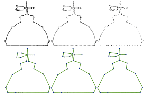
Alternatively to calling run(), one can call run_until() and specify the number of output vertices one wants to keep as illustrated in Figure 64.3.
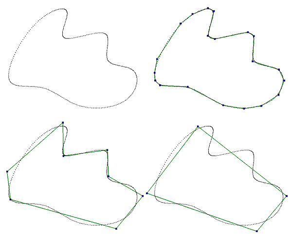
Finally, calling run_under_wasserstein_tolerance() allows the user to run the algorithm based on a distance criterion when the number of output edges is not known as illustrated in Figure 64.4.
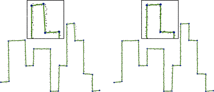
As noise and missing data may prevent the reconstructed shape to have sharp corners at the correct places, the algorithm offers a function to relocate all points of the reconstruction:
Note that these points coincide with the vertices of the underlying triangulation. This function can be called either after one run of simplification, or interleaved with several runs of simplification.
The new point locations are chosen such that the approximation of the output segments and isolated points to the input points is improved. More specifically, the relocation process iterates between computing the best transport plan given the current reconstruction, and relocating the triangulation vertices while keeping the current transport plan unchanged. The vertices are relocated so as to minimize the transport cost induced by the current transport plan [1].
The behavior of the algorithm is controlled via the following parameters.
During simplification of the internal triangulation some recursive edge flip operators are required to guarantee that the triangulation remain valid when applying a half edge collapse operator (see Figure 64.6). Calling set_use_flip(false) prevents the algorithm from using edge flips, yielding shorter computational times at the price of suboptimal results as not all edges can be considered for being collapsible.
An edge is relevant from the approximation point of view if (1) it is long, (2) approximates a large number of points (or a large amount of mass when points have mass attributes), and (3) has a small approximation error. More specifically, the notion of relevance is defined as \( m(e) * |e|^2 / cost(e) \), where \( m(e) \) denotes the mass of the points approximated by the edge, \( |e| \) denotes the edge length and \( cost(e) \) its approximation error. As the error is defined by mass time squared distance the relevance is unitless. The default value is 1, so that all edges approximating some input points are considered relevant. A larger relevance value provides us with a means to increase resilience to outliers.
By default the simplification relies upon an exhaustive priority queue of half edge collapse operators during decimation. For improved efficiency, a parameter sample size strictly greater than 0 switches to a multiple choice approach, i.e., a best-choice selection in a random sample of edge collapse operators, of size sample size. A typical value for the sample size is 15, but this value must be enlarged when targeting a very coarse simplification.
In addition to the global relocation function described above, an optional parameter of the constructor of the Optimal_transportation_reconstruction_2 class provides a means to relocate the points locally after each edge collapse operator (possibly combined with edge flips). Locally herein means that only the vertices of a local stencil in the triangulation around the each edge collapse operator are relocated, with a process similar to the one described above in the global relocation function. The local stencil is chosen as the one-ring neighborhood of the vertex remaining after collapsing an edge. The relocation process being iterative, one parameter controls the number of relocation steps.
The verbose parameter, between 0 and 2, determines how much console output the algorithm generates. A 0 value generates no output to the standard output. A value greater than 0 generates output to the standard output std::cerr.
A virtue of the algorithm is its robustness to noise and outliers. Figure 64.7 shows that the output of the algorithm is robust in the sense that it is hardly affected by noise and/or outliers, as long as the density of outliers is small compared to the density of the input points.
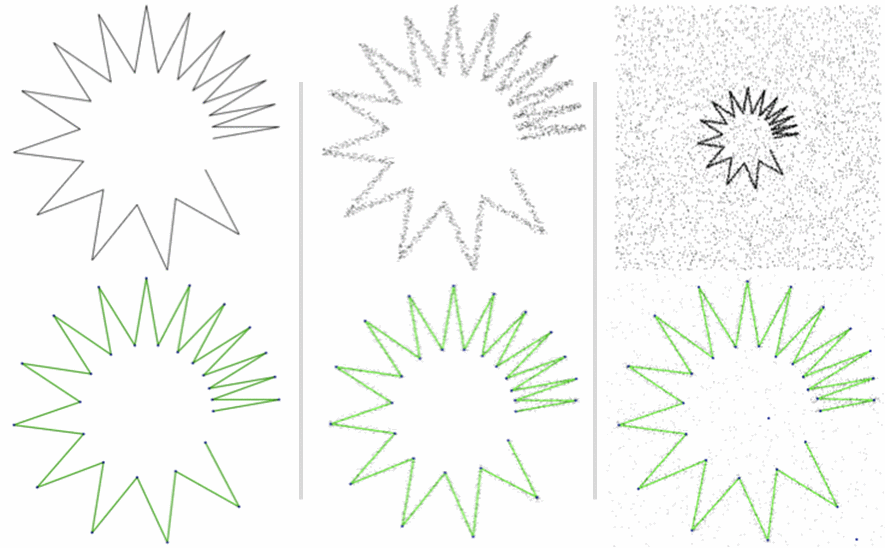
Figure 64.8 illustrates the behavior of the algorithm on a point set with uniform mass attributes, versus variable density. As the algorithm gives more importance to densely sampled areas, this translates into smaller edges on densely sampled areas. On sparsely sampled areas the algorithm initially approximates each point by one isolated vertex, then progressively approximates the points with edges.
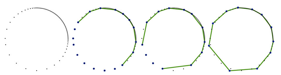
Figure 64.9 depicts an input point set sampling a set of line segments and a solid area. Depending on the targeted number of points in the output, the solid area is approximated by a set of evenly sampled isolated vertices.
The mass attributes provides a means to adjust the importance given to each point for approximation. Figure 64.10 depicts a reconstruction from a gray level image after thresholding, where the gray level of the pixels are used as mass attribute.
The task addressed here is to reconstruct a shape from a noisy point set \( S \) in \( \mathbb{R}^2 \), i.e., given a set of points in the plane, find a set of points and segments (more formally, a 0-1 simplicial complex ) which best approximates \( S \).
The approximation error is derived from the theory of optimal transportation between geometric measures [1]. More specifically, the input point set is seen as a discrete measure, i.e., a set of pointwise masses. The goal is to find a 0-1 simplicial complex where the edges are the support of a piecewise uniform continuous measure (i.e., a line density of masses) and the vertices are the support of a discrete measure. Approximating the input point set in our context translates into approximating the input discrete measure by another measure composed of line segments and points.
Intuitively, the optimal transportation distance (Wasserstein-2 distance in our context) measures the amount of work that it takes to transport the input measure onto the vertices and edges of the triangulation, where the measure is constrained to be uniform (and greater or equal to zero) on each edge, and just greater or equal to zero on each vertex. Note that the Wasserstein distance is symmetric.
When all vertices of the triangulation coincide with the input points (after full initialization) the total transport cost is zero as each input point relocates to a vertex at no cost, and the reconstruction is made of isolated vertices only.
Assume for now that the input point set is composed of 10 points (each with mass 1) uniformly sampled on a line segment, and that the triangulation contains a single edge coinciding with the line segment. Although the (one-sided Euclidean) distance from the points to the edge is zero (the converse being not zero), the Wasserstein distance from the points to the edge is non zero, as we constrain the mass density of the edge to be uniform, and the total mass (integral of density) of the edge to equal 10, i.e., the total mass of the input points. The input points should hence be transported tangentially on the edge in order to match the uniform density, the optimal transport plan for the input points being described as smaller line segments with equal lengths, covering the edge.
If one now samples uniformly 20 points on the same edge (each with mass 0.5) the Wasserstein distance is smaller (albeit the total mass is 10 as before), as the transport plan is described by smaller line segments. In a slightly different configuration where the 20 input points have different masses, the optimal transport plan is described by small line segments whose length is proportional to the mass of the associated input point. When the input points are not strictly on the edge, the transport plan has both tangential and normal components.
In other words, one approximates well the input points by a single edge when the input points are densely and uniformly sampling that edge. Beyond symmetry, one virtue of the Wasserstein distance is thus to quantize both the deviation from the points to the edge, and the non-uniformity of the points on that edge. This distance is also resilient to outliers (points far from the edge) when the mass of these outliers is small compared to the total mass of the input points.
The algorithm performs a fine to coarse simplification of a triangulation. It starts by constructing a box around the input points \(S\) and computes the Delaunay Triangulation \( T_0 \) on all or a subset of \( S \). \( T_0 \) is the first output simplex, which is simplified in subsequent iterations by repeated edge collapses. To chose the next edge, an edge collapse operator is simulated for all feasible edges, i.e., for edges which introduce neither overlaps nor fold-overs in the triangulation. The next edge \( e \) for collapse is chosen according to the overall cost of the transportation plan for \( T \setminus e \), where the cheapest overall cost is preferred. Since disregarding edges which do not preserve the embedding of the triangulation can severely affect the performance of the greedy approach to optimal transport, the collapse operator is modified by adding a local flip procedure which makes every edge collapsible.
The transportation plan is approximated by assigning each input point temporarily to the closest simplex edge. After this partitioning of the input points w.r.t. the edges, all the points temporarily assigned to a given edge are being assigned to it permanently if and only if the corresponding transportation costs are less than the transportation cost for each of the two end vertices of the edge. Otherwise each of the points is assigned to the cheapest of the two vertices. This process of edge collapse and transportation plan update is repeated until the desired number of vertices, specified by the users, has been reached.
At the end of the process, the edges which carry little mass can be filtered out and the remaining relevant edges and isolated vertices are reported as reconstructing the input shape.
This package is the result of the work of Ivo Vigan during the 2014 season of the Google Summer of Code. He has been mentored by Clément Jamin, Pierre Alliez and Fernando de Goes. The code is based on an initial research code written by Pierre Alliez and Fernando de Goes in 2010, for a paper published at the EUROGRAPHICS Symposium on Geometry Processing 2011 [1].
 1.8.13