

|
CGAL 5.4 - 2D Triangulations on the Sphere
|
|
CGAL 5.4 - 2D Triangulations on the Sphere
|
This chapter describes two-dimensional triangulations on the sphere. It is organized as follows:
Denote by \( \mathbb{S(c, r)}\) the two-dimensional sphere embedded in the Euclidean space \( \mathbb{R}^3\), with center c and radius r, that is \( \mathbb{S(c, r)} = \left\{ x \in \mathbf{R}^3 : \left\| x - c \right\| = r \right\} \). When the parameters c and r are not important, they will be omitted and \( \mathbb{S}\) will be used directly. Given a set \( \mathcal{P}\) of points on \( \mathbb{S(c, r)}\), a two-dimension triangulation of \( \mathcal{P}\) can be described as a two-dimensional simplicial complex that is pure, connected, and without singularity whose vertices are exactly the points in \( \mathcal{P}\) (see the complete definition in the package 2D Triangulations).
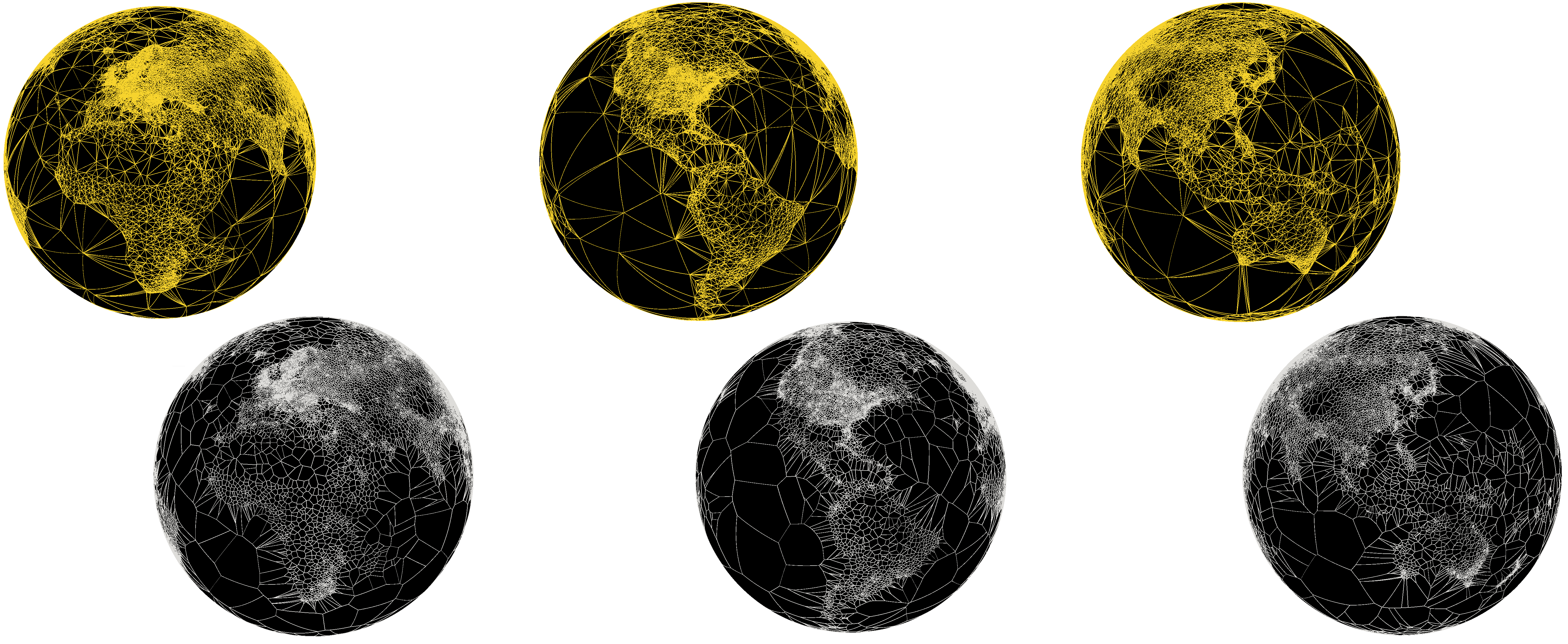
In \( \mathbb{R}^2\), a Delaunay triangulation is a two-dimension triangulation that satisfies the empty circle property (also called Delaunay property): the circumscribing circle of any facet of the triangulation contains no point in its interior. This definition naturally extends to the two-dimensional sphere, as illustrated in the figure below.
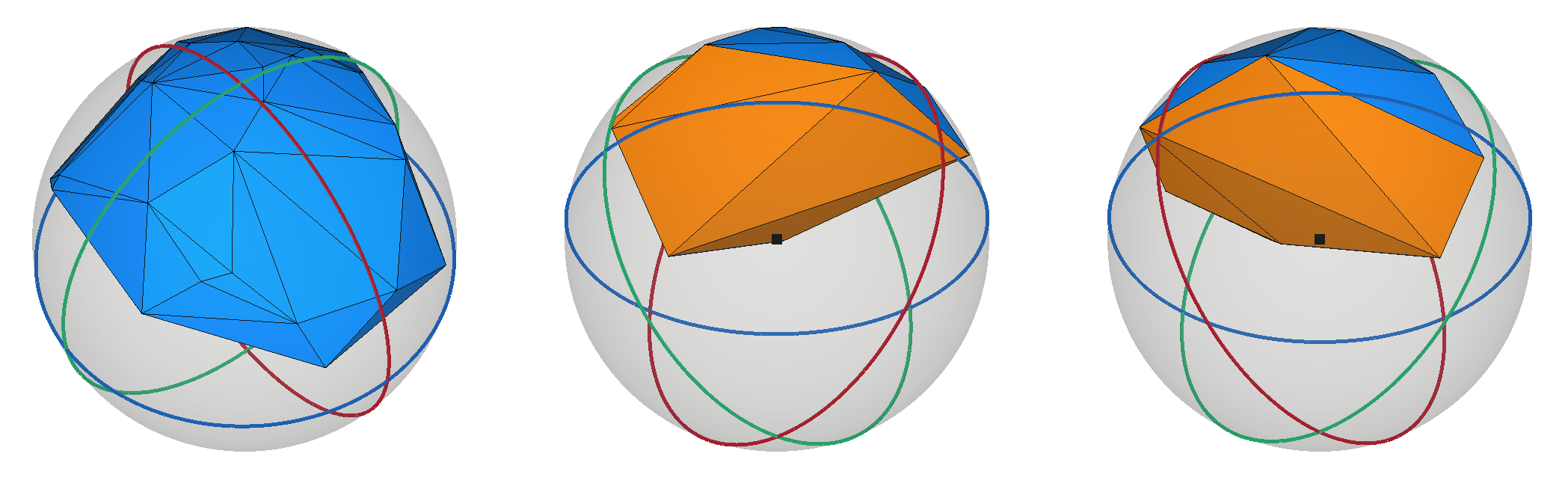
A particularity of Delaunay triangulations on \( \mathbb{S}\) is that the Delaunay property test can be reduced to a simple orientation test in the three-dimensional space: indeed, the circumscribing circle of a Delaunay face is the intersection of the plane passing through the three vertices of the face with \( \mathbb{S}\), and determining whether a fourth point q is within the circumscribing circle or not is equivalent to checking whether q is above or below the said supporting plane.
The theoretical definition of Delaunay triangulations in the previous section assumes that points in \( \mathcal{P}\) lie exactly on the sphere. In a real world however, one usually does not manipulate points that lie exactly on \( \mathbb{S}\) because the chosen number type is not able to represent square roots exactly, such as \( \mathtt{float}\), or \( \mathtt{double}\). Some specific number types are able to represent exactly all points on the sphere, for example the class CORE::Expr, but this comes with the drawback of a substantially higher computational cost.
This lack of exact representation is an obvious problem as the interpretation of the Delaunay property as an orientation test does not stand if points do not lie in a convex position.
This gap between the theoretical and the practical settings was addressed by Caroli et al. [1] : the solution is to use a regular triangulation, which is a generalization of the Delaunay triangulation to sets of weighted points (see 2D Regular Triangulations for more information). A weighted point \((p,w)\) of \( \mathbb{R}^2\) can naturally be seen as as a circle with center \( p\) and radius \( r\) such that \( r^2 = w\) and similarly to Delaunay triangulations and the definition of regular triangulations in \( \mathbb{R}^2\) can be naturally extended to circles on \( \mathbb{S}\). Given a set of points \( \mathcal{P}_3\) living in \( \mathbb{R}^3\), Caroli et al. compute a regular triangulation of the set of weighted points \( \mathcal{P}_w\) where the weighted points of \( \mathcal{P}_w\) are the projection of the points of \( \mathcal{P}_3\) onto \( \mathbb{S}\), and whose weights are based on the projection distance. Furthermore, they show that if the Euclidean distance between the points of \( \mathcal{P}_w\) is sufficiently large, and if the points are sufficiently close to the sphere, then the Delaunay triangulation of the Delaunay triangulation of \( \mathcal{P}_3\) is exactly the regular triangulation of \( \mathcal{P}_w\). As a consequence is that one can manipulate 3D points that are not exactly on the sphere, and it possible to build the Delaunay triangulation without taking the weights into account, as long as the points are sufficiently far from each other.
Caroli et al. et provide bounds on this separation criterion for the case of the \( \mathtt{double}\) number type: two points must be at least \( 2^{-25}r\) apart. This is a condition that is generally satisfied for most inputs: if \( r\) were for example the radius of the Earth, roughly 6300 kms, then the point separation requirement would be of the order of 1 meter.
The main class of this package is the class CGAL::Delaunay_triangulation_on_sphere_2; it represents a Delaunay triangulation on the sphere, and provides insertion and removal of vertices, as well as tools to draw the triangulation and its dual, the Voronoi diagram. The base of CGAL::Delaunay_triangulation_on_sphere_2 is the class CGAL::Triangulation_on_sphere_2. It represents a triangulation on the sphere, but does not support insertion or removal of vertices. Both classes are built on top of a data structure called the triangulation data structure. The triangulation data structure can be thought of as a container for the faces and vertices of the triangulation. This data structure also takes care of all the combinatorial aspects of the triangulation.
These triangulation classes are intentionally very similar to CGAL::Delaunay_triangulation_2 and CGAL::Triangulation_2 as both classes represent triangulations of a 2-manifold domain without boundary. As such, many details about the implementation are not repeated here, and complementary information can be found in the Sections Representation, Software Design, and Basic Triangulations of the package 2D Triangulations.
However, a significant departure from Euclidean 2D triangulations is the following: since the triangulation data structure represents a 2-manifold without boundary, it is necessary for 2D triangulations to introduce so-called infinite faces to complete the "real" triangulation (see The Set of Faces). On the sphere, this trick is not necessary as the triangulation itself is already a 2-manifold without boundary.
There is an exception to the previous statement: in degenerate configurations where all points lie on the same hemisphere, the Delaunay triangulation on the sphere theoretically has a border. Internally however, the triangulation data structure must remain a 2-manifold at all time. To ensure this property, fictitious faces referred to as ghost faces are added. These faces are characterized by the fact that the center of the sphere does not (strictly) lie on the positive side of the supporting plane of the face. Conversely, faces that are not ghost faces are called solid faces, and edges of such faces are solid edges.
Two traits classes are offered with this package as models of the concept DelaunayTriangulationOnSphereTraits_2:
CGAL::Delaunay_triangulation_on_sphere_traits_2: This is the simplest possible traits, which represents points on sphere directly as 3D points. If its kernel template parameter cannot represent all points on the sphere exactly, it employs the solution described in Section Representation of a Point on the Sphere to determine whether a point should be considered on the sphere, or too close to an existing vertex. CGAL::Projection_on_sphere_traits_3: This traits class utilizes a custom internal point type for points on the sphere: given a point p in 3D space, this traits class manipulates directly its projection on the sphere (that is, the intersection of the sphere and the segment with endpoints p and the center of the sphere). Consequently, all points to be inserted are on the sphere. This traits enable manipulating points that are not on the sphere, but whose triangulation on the sphere is still interesting, such as geographical coordinates with altitude. Both these classes are templated by a kernel. The choice of this kernel is important to ensure a correct result: for the construction of triangulations to be safe, the kernel should provide exact predicates (for example, CGAL::Exact_predicates_inexact_constructions_kernel). In addition, some auxiliary functions such as those used in the construction of the Voronoi diagram require creating new geometric points; as such, a kernel offering an exact representation of points on the sphere and exact constructions (for example, CGAL::Exact_predicates_exact_constructions_kernel_with_sqrt) should be used if one wants to avoid otherwise inevitable numerical approximations.
Mostly by convention with other triangulations, the dimension of a triangulation on the sphere is defined as follows:
-2, if the triangulation is empty; -1, if the triangulation contains a single vertex; 0, if the triangulation contains exactly two vertices; 1, if the triangulation contains at least three coplanar vertices (which do not necessarily lie on a great circle); 2, if the triangulation contains at least four non-coplanar vertices. Note that a triangulation of dimension 1 is just a polygon drawn on a circle. The polygon is not triangulated itself. Thus the triangulation of dimension 1 consists of a planar polygon and has no faces.
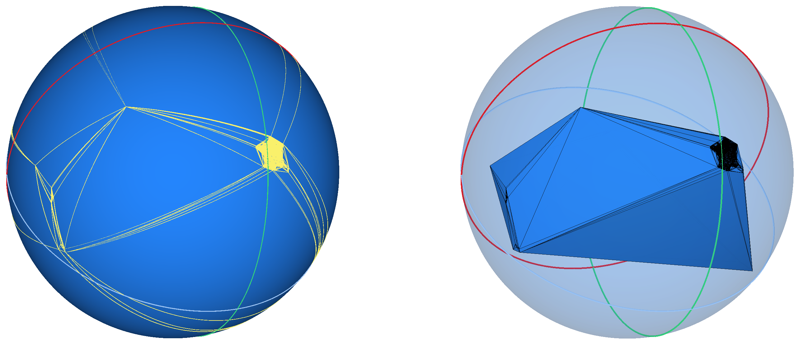
The descriptions of Delaunay (and regular) triangulations over \( \mathbb{S}\) have so far been mostly combinatorial. The question of the geometrical embedding of the simplices of the triangulation is also interesting. The two natural embedding of edges and faces of a triangulation of a set of points on \( \mathbb{S}\) are to use either straight simplex, that is using three-dimensional segments and triangles for the edges and faces of the triangulation, or to use a curved embedding, where the edges are arc segments of great circles over \( \mathbb{S}\). In the latter choice, the geometrical embedding of the face is defined implicitely by its three edges.
Both choices are available to users, for example using either Triangulation_on_sphere_2::segment() or Triangulation_on_sphere_2::segment_on_sphere(). Similar choices are available in the construction of the dual, the Voronoi diagram.
The following example uses the simplest traits class provided in this package. It demonstrates how to iteratively insert a few points, and how the dimension and the data structure of the triangulation evolve with these insertions.
File Triangulation_on_sphere_2/triang_on_sphere.cpp
The following example illustrates the limitation of using a kernel with inexact representation of points on the sphere and the rejection of a point for being too close to an already existing vertex. A kernel providing exact representation is also shown to be able to insert these two extremely close points.
File Triangulation_on_sphere_2/triang_on_sphere_exact.cpp
In this example, the use of the projection traits class is illustrated.
File Triangulation_on_sphere_2/triang_on_sphere_proj.cpp
The following example demonstrates how to insert a range of points at once. This enables an internal algorithm to sort the set of points to ensure locality when inserting points, which greatly speeds up the insertion.
File Triangulation_on_sphere_2/triang_on_sphere_range.cpp
Prototype code implementing the publication of Caroli et al. [1] was developed over the two internships of Oliver Rouiller and Claudia Werner at Inria, under the supervision of Monique Teillaud and with the help of Sébastien Loriot. Based on this prototype, Mael Rouxel-Labbé developed the initial version of this package.
The work was partially supported by the grant ANR-17-CE40-0033 of the French National Research Agency ANR (project SoS) and INTER/ANR/16/11554412/SoS of the Luxembourg National Research fund FNR.
 1.8.13