This package allows the estimation of local differential quantities of a surface from a point sample, given either as a mesh or as point cloud.
Note that this package needs the third party libraries Lapack and Blas to be installed to compile the example code.
42.1 Introduction
42.1.1 Overview
Consider a sampled smooth surface, and assume we are given a collection of points about a given sample . We aim at estimating the differential properties up to any fixed order of the surface at point from the point set - we denote . More precisely, first order properties correspond to the normal or the tangent plane; second order properties provide the principal curvatures and directions, third order properties provide the directional derivatives of the principal curvatures along the curvature lines, etc. Most of the time, estimating first and second order differential quantities is sufficient. However, some applications involving shape analysis require estimating third and fourth order differential quantities. Many different estimators have been proposed in the vast literature of applied geometry [Pet01] (section 3, page 7), and all of them need to define a neighborhood around the point at which the estimation is computed. Our method relies on smooth differential geometry calculations, carried out on smooth objects fitted from the sample points. Datasets amenable to such a processing are naturally unstructured point clouds, as well as meshes - whose topological information may be discarded.
Estimating differential properties from discrete date always raises a philosophical issue. On one hand, estimating differential quantities subsumes a smooth surface does exist. In this spirit one wishes to recover its differential properties, so that any estimation method must come with an asymptotic convergence analysis of the results returned. For the method developed in this CGAL package, the interested will find such an analysis in [CP05a], (Theorem 3) - it should be stressed the error bounds proved therein are optimal.
On the other hand, any estimation method may be applied to arbitrarily data - surface unknown, surface piecewise smooth etc. In such a case, no analysis can be carried out, and it is up to the users to check the results match their needs.
Unlike most of the CGAL packages, this package uses approximation methods and is not intended to provide an exact canonical result in any sense. This is why internal computations are performed with a number type possibly different from that of the input data, even if for convenience the results are returned with this original number type. A reasonable choice for this internal number type is for example the double type.
42.1.2 Smooth Surfaces, -Jets and the Monge Form
To present the method, we shall need the following notions. Consider a smooth surface. About one of its points, consider a coordinate system whose -axis does not belong to the tangent space. In such a frame, the surface can locally be written as the graph of a bivariate function. Letting stand for higher order terms, one has :
The degree polynomial is the Taylor expansion of the function , and is called its -jet. Notice that a -jet contains coefficients.
Recall that an umbilical point of a surface - or umbilic for short, is a point where both principal curvatures are identical. At any point of the surface which is not an umbilic, principal directions are well defined, and these (non oriented) directions together with the normal vector define two direct orthonormal frames. If is a unit vector of direction , there exists a unique unit vector so that is direct; and the other possible frame is . Both these coordinate systems are known as the Monge coordinate systems. In both these systems, the surface is said to be given in the Monge form and its jet has the following canonical form :
The coefficients are the principal curvatures, are the directional derivatives of along their respective curvature line, while are the directional derivatives of along the other curvature lines.
The Monge coordinate system can be computed from any -jet (), and so are the Monge coefficients. These informations characterize the local geometry of the surface in a canonical way, and are the quantities returned by our algorithm.
42.1.3 Algorithm
Based on the above concepts, the algorithm consists of 4 steps.- We perform a Principal Component Analysis (PCA) on . This analysis outputs three orthonormal eigenvectors and the associated eigenvalues. The fitting basis consists of these three vectors so that the vector associated to the smallest eigenvalue is the last vector of the basis. (Indeed, if the surface is well sampled, one expects the PCA to provide one small and two large eigenvalues, the eigenvector associated to the small one approximating the normal vector.)
- We perform a change of coordinates to move the samples into the coordinate system of the fitting basis and with origin the point at which the estimation is sought. We then resort to polynomial fitting, so as to either interpolate or approximate the -jet of the surface in this coordinate system. This bivariate polynomial approximation reduces to linear algebra operations.
- From the fitted -jet, we compute the Monge basis .
- Finally, we compute the Monge coefficients : .
Further details can be found in section 42.4 and in [CP05a] (section 6).
42.1.4 Degenerate Cases
As usual, the fitting procedure may run into (almost) degenerate cases:
- Due to poor sampling, the PCA used to determine a rough normal
vector may not be good. The nearer this direction to the tangent
plane the worse the estimation.
- As observed in [CP05a] (section 3.1), the interpolating problem is not poised if the points project, into the fitting frame, onto an algebraic curve of degree . More generally, the problem is ill poised if the condition number is too large.
42.2 Software Design
42.2.1 Options and Interface Specifications
The fitting strategy performed by the class Monge_via_jet_fitting requires the following parameters:
- the degree of the fitted polynomial (),
- the degree of the Monge coefficients sought, with min,
- a range of input points on the surface, with the precondition that . Note that if , interpolation is performed; and if , approximation is used.
42.2.2 Output
As explained in Section 42.1, the output consists of a coordinate system, the Monge basis, together with the Monge coefficients which are stored in the Monge_form class. In addition, more information on the computational issues are stored in the Monge_via_jet_fitting class.
The Monge_form class provides the following information.
- Origin. This is the point on the fitted polynomial surface
where the differential quantities have been computed. In the
approximation case, it differs from the input point : it is the
projection of onto the fitted surface following the -direction
of the fitting basis.
- Monge Basis. The Monge basis is orthonormal
direct, and the maximal, minimal curvatures are defined wrt this
basis. If the user has a predefined normal (e.g. the sample
points come from an oriented mesh) then if then max-min
is correct; if not, i.e. , the user should switch to the
orthonormal direct basis with the
maximal curvature and the minimal curvature
. If or is small, the orientation of the
surface is clearly ill-defined, and the user may proof-check the
samples used to comply with its predefined normal.
- Monge Coefficients.
The coefficient of the Monge form is for .
In addition, the class Monge_via_jet_fitting stores
- the condition number of the fitting system,
- the coordinate system of the PCA (in which the fitting is performed).
42.2.3 Template Parameters
Template parameter DataKernel
This concept provides the types for the input sample points, together with vectors and a number type. It is used as template for the classe Monge_via_jet_fitting<DataKernel, LocalKernel = Cartesian<double>, SvdTraits = lapack_svd> . Typically, one can use CGAL::Cartesian<double>.
Template parameter LocalKernel
This is a parameter of the class Monge_via_jet_fitting<DataKernel, LocalKernel = Cartesian<double>, SvdTraits = lapack_svd>. This concept defines the vector and number types used for local computations and to store the PCA basis data.Input points of type DataKernel::Point_3 are converted to LocalKernel::Point_3. For output of the Monge_form class, these types are converted back to Data_Kernel ones. Typically, one can use CGAL::Cartesian<double> which is the default.
Template parameter SvdTraits
This concept provides the number, vector and matrix types for algebra operations required by the fitting method in Monge_via_jet_fitting<DataKernel, LocalKernel = Cartesian<double>, SvdTraits = lapack_svd> . The main method is a linear solver using a singular value decomposition.
Compatibility requirements
To solve the fitting problem, the sample points are first converted from the DataKernel to the LocalKernel (this is done using the CGAL::Cartesian_converter). Then change of coordinate systems and linear algebra operations are performed with this kernel. This implies that the number types LocalKernel::FT and SvdTraits::FT must be identical. Second the Monge basis and coefficients, computed with the LocalKernel, are converted back to the DataKernel (this is done using the CGAL::Cartesian_converter and the CGAL::NT_converter).
42.3 Examples
42.3.1 Single Estimation about a Point of a Point Cloud
The first example illustrates the computation of the local differential quantities from a set of points given in a text file as input. The first point of the list is the one at which the computation is performed. The user has to specify a file for the input points and the degrees and .
File: examples/Jet_fitting_3/Single_estimation.cpp
#include <CGAL/Cartesian.h>

#ifndef CGAL_USE_LAPACK
int main()
{
  std::cerr << "Skip since LAPACK is not installed" << std::endl;
  std::cerr << std::endl;
  return 0;
}
#else

#include <fstream>
#include <vector>

#include <CGAL/Monge_via_jet_fitting.h>
typedef double                   DFT;
typedef CGAL::Cartesian<DFT>     Data_Kernel;
typedef Data_Kernel::Point_3     DPoint;
typedef CGAL::Monge_via_jet_fitting<Data_Kernel> My_Monge_via_jet_fitting;
typedef My_Monge_via_jet_fitting::Monge_form     My_Monge_form;

int main(int argc, char *argv[])
{
  //check command line
  if (argc<4)
    {
      std::cout << " Usage : " << argv[0]
                << " <inputPoints.txt> <d_fitting> <d_monge>" << std::endl;
      return 0;
    }
  //open the input file
  std::ifstream inFile( argv[1]);
  if ( !inFile )
    {
      std::cerr << "cannot open file for input\n";
      exit(-1);
    }
  //initalize the in_points container
  double x, y, z;
  std::vector<DPoint> in_points;
  while (inFile >> x) {
    inFile >> y >> z;
    DPoint p(x,y,z);
    in_points.push_back(p);
  }
  inFile.close();
  // fct parameters
  size_t d_fitting = std::atoi(argv[2]);
  size_t d_monge = std::atoi(argv[3]);

  My_Monge_form monge_form;
  My_Monge_via_jet_fitting monge_fit;
  monge_form = monge_fit(in_points.begin(), in_points.end(), d_fitting, d_monge);

  //OUTPUT on std::cout
  CGAL::set_pretty_mode(std::cout);
  std::cout << "vertex : " << in_points[0] << std::endl
	    << "number of points used : " << in_points.size() << std::endl
	    << monge_form;
  std::cout  << "condition_number : " << monge_fit.condition_number() << std::endl
	     << "pca_eigen_vals and associated pca_eigen_vecs :"  << std::endl;
  for (int i=0; i<3; i++)
    std::cout << monge_fit.pca_basis(i).first << std::endl
	      << monge_fit.pca_basis(i).second  << std::endl;
  return 0;
}
#endif //CGAL_USE_LAPACK
42.3.2 On a Mesh
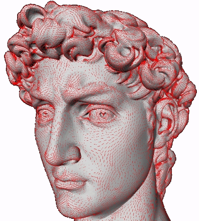
The second example (cf Mesh_estimation.cpp in the example directory) illustrates the computation of local differential quantities for all vertices of a given mesh. The neighborhood of a given vertex is computed using rings on the triangulation. Results are twofold:- a human readable text file featuring the Monge_form and numerical informations on the computation : condition number and the PCA basis;
- another text file which may be visualised with the demo program introspect-qt (experimental CGAL package) displaying the Monge basis at each vertex of the mesh.
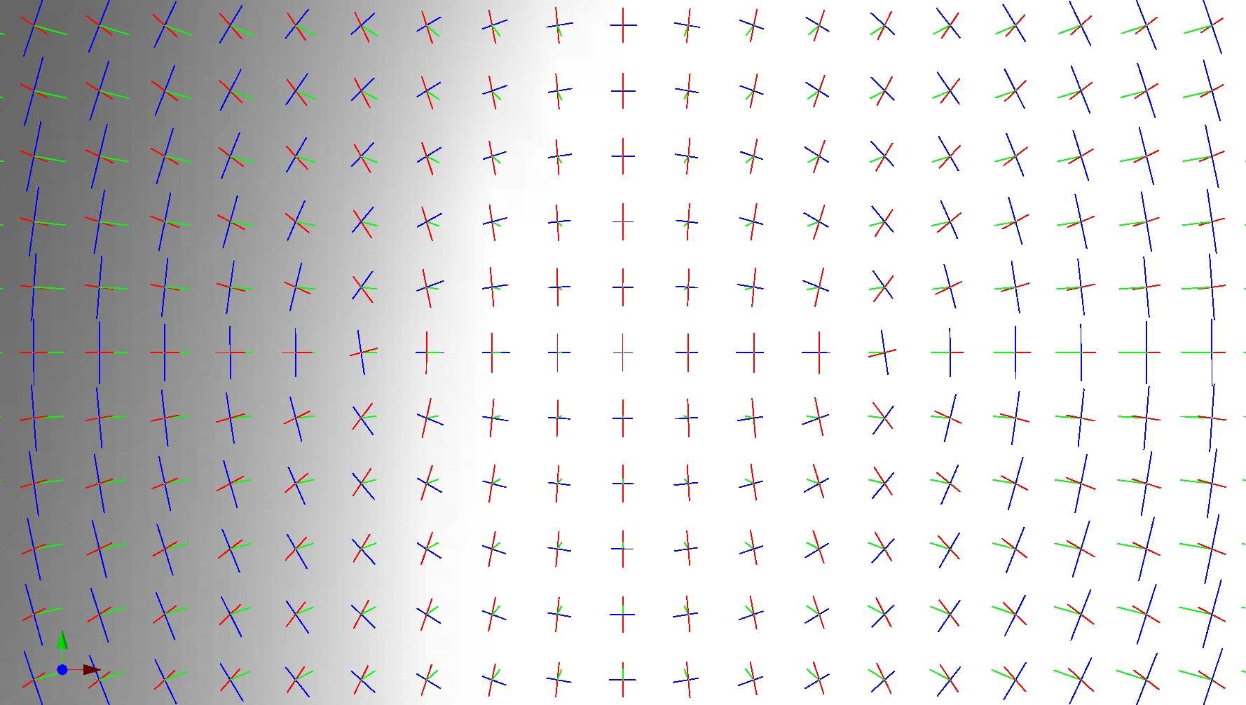
Figs. 42.1 and 42.2 provide illustrations of principal directions of curvature.
Figure 42.2: Principal directions of curvature and normals at vertices of a mesh of the graph of the function .

| advanced |

|
42.4 Mathematical and Algorithmic Details
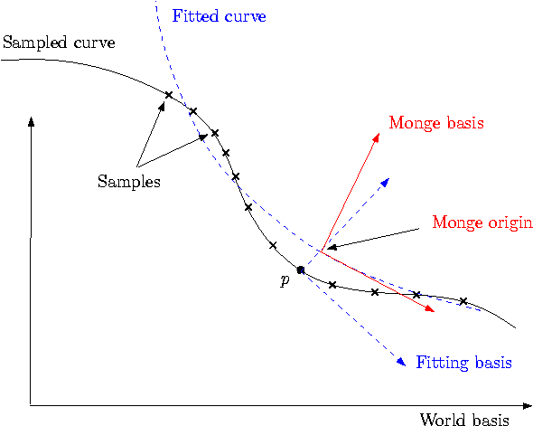
In this Section, we detail the mathematics involved, in order to justify the design choices made. To begin with, observe the fitting problem involves three relevant direct orthonormal basis: the world-basis , the fitting-basis , the Monge basis .Figure 42.3: The three bases involved in the estimation.
42.4.1 Computing a Basis for the Fitting
Input : samples
Output : fitting-basis
Performing a PCA requires diagonalizing a symmetric matrix. This analysis gives an orthonormal basis whose -axis is provided by the eigenvector associated to the smallest eigenvalue.1 Note one may have to swap the orientation of a vector to get a direct basis.
Let us denote the matrix that changes coordinates from the world-basis to the fitting-basis . The rows of are the coordinates of the vectors in the world-basis. This matrix represents a orthogonal transformation hence its inverse is its transpose. To obtain the coordinates of a point in the fitting-basis from the coordinates in the world-basis, one has to multiply by .
As mentioned above, the eigenvalues are returned, from which the sampling quality can be assessed. For a good sampling, the eigenvector associated to the smallest eigenvalue should roughly give the normal direction.
42.4.2 Solving the Interpolation / Approximation Problem
Input : samples, fitting-basis
Output : coefficients
of the bivariate fitted polynomial in the fitting-basis
Computations are done in the fitting-basis and the origin is the point . First, one has to transform coordinates of sample points with a translation () and multiplication by .
The fitting process consists of finding the coefficients of the degree polynomial
Denote the coordinates of the sample points of . For interpolation the linear equations to solve are , and for approximation one has to minimize . The linear algebra formulation of the problem is given by
The equations for interpolation become . For approximation, the system is solved in the least square sense, i.e. one seeks the vector such that argmin.
In any case, there is a preconditioning of the matrix so as to improve the condition number. Assuming the , are of order , the pre-conditioning consists of performing a column scaling by dividing each monomial by - refer to Eq. (42.4.2). Practically, the parameter is chosen as the mean value of the and . In other words, the new system is with the diagonal matrix , so that the solution of the original system is .
There is always a single solution since for under constrained systems we also minimize . The method uses a singular value decomposition of the matrix , where is a orthogonal matrix, is a orthogonal matrix and is a matrix with the singular values on its diagonal. Denote the rank of , we can decompose The number , which is the number of non zero singular values, is strictly lower than if the system is under constrained. In any case, the unique solution which minimize is given by :
One can provide the condition number of the matrix (after preconditioning) which is the ratio of the maximal and the minimal singular values. It is infinite if the system is under constrained, that is the smallest singular value is zero.
Implementation details. We assume a solve function is provided by the traits SvdTraits. This function solves the system MX=B (in the least square sense if M is not square) using a Singular Value Decomposition and gives the condition number of M.
Remark: as an alternative, other methods may be used to solve the
system. A decomposition can be substituted to the . One can
also use the normal equation and apply methods for square
systems such as , or Cholesky since is symmetric
definite positive when has full rank.
The advantages of the
is that it works directly on the rectangular system and gives the
condition number of the system. For more on these alternatives, see
[GvL83] (Chap. 5).
42.4.3 Principal Curvature / Directions
Input : coefficients of the fit ,
fitting-basis
Output : Monge basis wrt fitting-basis and world-basis
In the fitting basis, we have determined a height function expressed by Eq. (42.4.2). Computations are done in the fitting-basis. The partial derivatives, evaluated at , of the fitted polynomial are Expanding Eq. (42.4.2) yields:
- The origin, that is the point of the fitted surface where the estimation is performed, is .
- The normal is .
- Curvature related properties are retrieved resorting to standard differential calculus [dC76] (Chap. 3). More precisely, the Weingarten operator is first computed in the basis of the tangent plane . We compute an orthonormal basis of the tangent plane using the Gram-Schmidt algorithm, and then we compute Weingarten in this basis (applying a change of basis with the matrix ). In this orthonormal basis, the matrix of the Weingarten map is symmetric and we diagonalize it. One finally gets the principal curvatures which are the eigenvalues of , and the associated principal directions. This gives an orthonormal direct basis . Let us denote the matrix to change coordinates from the fitting-basis to the Monge basis. Its rows are the coordinates of the vectors in the fitting-basis. It is an orthogonal matrix . The Monge basis expressed in the world-basis is obtained by multiplying the coordinates of in the fitting-basis by , (the same holds for the origin point which has in addition to be translated by , i.e. the coordinates of the origin point are .
42.4.4 Computing Higher Order Monge Coefficients
Input : coefficients of the fit, Monge basis wrt fitting-basis ()
Output : third and fourth order coefficients of Monge
We use explicit formula. The implicit equation of the fitted polynomial surface in the fitting-basis with origin the point is with
The equation in the Monge basis is obtained by substituting by . Denote this implicit equation. By definition of the Monge basis, we have locally (at )
and the Taylor expansion of at are the Monge coefficients sought. Let us denote the partial derivatives evaluated at the origin of and by and . One has , and , . The partial derivative of order of depends on the matrix and the partial derivatives of order at most of . The third and fourth order coefficients of are computed with the implicit function theorem. For instance :

| advanced |

|
Footnotes
| 1 | Another possibility is to choose as z-axis the axis of the world-basis with the least angle with the axis determined with the PCA. Then the change of basis reduces to a permutation of axis. |
Navigation: Up, Table of Contents, Package Overview, Bibliography, Index, Title Page , Acknowledging CGAL