Chapter 71
Kinetic Data Structures
Daniel Russel
Table of Contents
Lets say you want to maintain a sorted list of items (each item is
associate with a real number key). You can imagine placing each of the
items on the point on the real line corresponding to its key. Now, let
the key for each item change continuously (i.e. no jumps are allowed).
As long as no two (consecutive) items cross, the sorted order is
intact. When two items cross, they need to be exchanged in the list and then
the sorted order is once again correct. This is a trivial example of a
kinetic data structure. The key observation is that the combinatorial
structure which is maintained changes at discrete times (events) even
though the basic building blocks are changing continuously.
This chapter describes a number of such kinetic data structures
implemented using the Kinetic framework described in
Chapter 72. We first, in
Section 71.2 introduce kinetic data structures and
sweepline algorithms. This section can be skipped if the reader is
already familiar with the area. The next sections,
Section 71.2.1 and Section 71.3 introduce
the terms and give an overview of the framework. They are recommended
reading for all readers, even if you are just using provided kinetic
data structures. We then present kinetic data structures for Delaunay
triangulations in two and three dimensions in
Section 71.4.
If you are already familiar with kinetic data structures and know what
you want to do, you might want to first take a look at the next section
Section 71.1 which covers quick hints.
71.1 Quick Hints
This section gives quick answers to some questions people might have.
It presumes knowledge of kinetic data structures and this framework.
How do I store extra information allow with, for example, a kinetic Point_2?
See the example
Kinetic_framework/defining_a_simulation_traits.cpp to see how
to define a new SimulationTraits class where the
Active-Objects-Table contains extra data along with the point.
Where is the best place to look if I want to write my own kinetic data structure?
We provide two simple kinetic data structures, first most trivial is
Kinetic_framework/trivial_kds.cpp and a slightly more
complicated one is:
#include <CGAL/Kinetic/Sort.h>
How can I use kinetic data structures to update Delaunay triangulations?
We are working on that one, but you will have to wait.
71.2 An Overview of Kinetic Data Structures and Sweep Algorithms
Kinetic data structures were first introduced in by Basch et. al. in
1997 [BGH97]. The idea stems from the observation that
most, if not all, computational geometry structures are built using
predicates - functions on quantities defining the geometric
input (e.g. point coordinates), which return a discrete set of
values. Many predicates reduce to determining the sign of a polynomial
on the defining parameters of the primitive objects. For example, to
test whether a point lies above or below a plane we compute the dot
product of the point with the normal of the plane and subtract the
plane's offset along the normal. If the result is positive, the point
is above the plane, zero on the plane, negative below. The validity of
many combinatorial structures built on top of geometric primitives can
be verified by checking a finite number of predicates of the geometric
primitives. These predicates, which collectively certify the
correctness of the structure, are called certificates. For a
Delaunay triangulation in three dimensions, for example, the
certificates are one InCircle test per facet of the
triangulation, plus a point plane orientation test for each facet or
edge of the convex hull.
The kinetic data structures approach is built on top of this view of
computational geometry. Let the geometric primitives move by replacing
each of their defining quantities with a function of time (generally a
polynomial). As time advances, the primitives trace out paths in
space called trajectories. The values of the polynomial
functions of the defining quantities used to evaluate the predicates now
also become functions of time. We call these functions
certificate functions. Typically, a geometric structure is valid when
all predicates have a specific non-zero sign. In the kinetic setting,
as long as the certificate functions maintain the correct sign as time varies,
the corresponding predicates do not change values,
and the original data structure remains correct. However, if
one of the certificate functions changes sign, the original structure
must be updated, as well as the set of certificate functions that
verify it. We call such occurrences events.
Maintaining a kinetic data structure is then a matter of determining
which certificate function changes sign next, i.e. determining which
certificate function has the first real root that is greater than the
current time, and then updating the structure and the set of
certificate functions. In addition, the trajectories of primitives are
allowed to change at any time, although C0-continuity of the
trajectories must be maintained. When a trajectory update occurs for
a geometric primitive, all certificates involving that primitive must
be updated. We call the collection of kinetic data structures,
primitives, event queue and other support structures a
simulation.
Sweepline algorithms for computing arrangements in d dimensions
easily map on to kinetic data structures by taking one of the
coordinates of the ambient space as the time variable. The kinetic
data structure then maintains the arrangement of a set of objects
defined by the intersection of a hyperplane of dimension d-1 with
the objects whose arrangement is being computed.
Time is one of the central concepts in a kinetic simulation. Just as
static geometric data structures divide the continuous space of all
possible inputs (as defined by sets of coordinates) into a discrete
set of combinatorial structures, kinetic data structures divide the
continuous time domain into a set of disjoint intervals. In each
interval the combinatorial structure does not change, so, in terms of
the combinatorial structure, all times in the interval are equivalent.
We capitalize on this equivalence in the framework in order to
simplify computations. If the primitives move on polynomial
trajectories and the certificates are polynomials in the coordinates,
then events occur at real roots of polynomials of time. Real numbers,
which define the endpoints of the interval, are more expensive to
compute with than rational numbers, so performing computations at a
rational number inside the interval is preferable whenever
possible. See Section 72.1.4 for an example of
where this equivalence is exploited.
71.2.1 Terms Used
- primitive
- The basic geometric types, e.g., the points of a
triangulation. A primitive has a set of coordinates.
- combinatorial structure
- A structure built on top of the
primitives. The structure does not depend directly on the
coordinates of the primitives, only on relationships between them.
- trajectory
- The path traced out by a primitive as time passes.
In other words how the coordinates of a primitive change with time.
- snapshot
- The position of all the primitives at a particular
moment in time.
- static
- Having to do with geometric data structures on
non-moving primitives.
- predicate
- A function which takes the coordinates of several
primitives from a snapshot as input and produces one of a discrete
set of outputs.
- certificate
- One of a set of predicates which, when all having
the correct values, ensure that the combinatorial structure is
correct.
- certificate function
- A function of time which is positive when
the corresponding certificate has the correct value. When the
certificate function changes sign, the combinatorial structure needs
to be updated.
- event
- When a certificate function changes sign and the
combinatorial structure needs to be updated.
71.3 An Overview of the Kinetic Framework
The provided kinetic data structures are implemented on top of the
Kinetic framework presented in Chapter 72. It is
not necessary to know the details of the framework, but some
familiarity is useful. Here we presented a quick overview of the
framework.
The framework is structured around five main concepts. See
Figure 71.1 for a schematic of how a kinetic data
structure interacts with the various parts. The main concepts are
- the Kinetic::Simulator. Models of this concept process events in
the correct order and audit kinetic data structures. There should be
one instance of a model of this concept per simulation.
- the Kinetic::Kernel. The structure of a
Kinetic::Kernel is analogous to the static Cgal (i.e.,
non-kinetic) kernels in that it defines a set of primitives and
functors which generate certificates from the primitives.
- the Kinetic::ActiveObjectsTable. Models of this concept hold a
collection of kinetic primitives in a centralized manner. This
structure centralizes management of the primitives in order to
properly disseminate notifications when trajectories change, new
primitives are added or primitives are deleted.
There is generally one instance of a model of this concept per simulation.
- the Kinetic::InstantaneousKernel. Models of this concept allow
existing non-kinetic Cgal data structures to be used on a snapshot
of kinetic data. As a result, pre-existing static structures can be
used to initialize and audit kinetic data structures.
- the Kinetic::FunctionKernel. This concept is the computational
kernel of our framework. Models of this concept are responsible for
representing, generating and manipulating the motional and
certificate functions and their roots. It is this concept that
provides the kinetic data structures framework with the necessary
algebraic operations for manipulating event times. The
Kinetic::FunctionKernel is discussed in detail in Section
72.2.
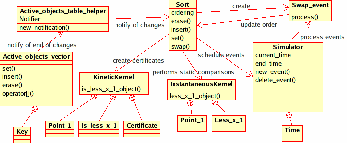
Figure 71.1: The figure shows the interaction between
the Kinetic::Sort<Traits, Visitor> kinetic data structure and
the various pieces of our package. Other, more complicated, kinetic
data structures will also use the Kinetic::InstantaneousKernel in order
to insert/remove geometric primitives and audit
themselves. Kinetic::Sort<Traits, Visitor> uses the sorting
functionality in the Stl instead.
For simplicity, we added an additional concept, that of
Kinetic::SimulationTraits, which wraps together a particular set of
choices for the above concepts and is responsible for creating
instances of each of the models. As a user of existing kinetic data
structures, this is the only framework object you will have to
create. The addition of this concept reduces the choices the user has
to make to picking the dimension of the ambient space and choosing
between exact and inexact computations. The model of
Kinetic::SimulationTraits creates an instance each of the
Kinetic::Simulator and Kinetic::ActiveObjectsTable. Handles for
these instances as well as instances of the Kinetic::Kernel
and Kinetic::InstantaneousKernel can be requested from the simulation
traits class. Both the Kinetic::Kernel and the
Kinetic::Simulator use the Kinetic::FunctionKernel,
the former to find certificate failure times and the later to operate
on them. For technical reasons, each supplied model of
Kinetic::SimulationTraits also picks out a particular type of
kinetic primitive which will be used by the kinetic data structures.
71.4 Using Kinetic Data Structures
There are five provided kinetic data structures. They are
- Kinetic::Sort<Traits, Visitor>
- maintain a list of points
sorted by x-coordinate.
- Kinetic::Delaunay_triangulation_2<Traits, Visitor, Triangulation>
- maintain the Delaunay triangulation of a set of
two dimensional points
- Kinetic::Delaunay_triangulation_3<Traits,Visitor, Triangulation>
- maintain the Delaunay triangulation of a set of
three dimensional points.
- Kinetic::Regular_triangulation_3<Traits, Visitor, Triangulation>
- maintain the regular triangulation of a set of waiting
three dimensional points.
- Kinetic::Enclosing_box_2<Traits>,
Kinetic::Enclosing_box_3<Traits>
- restrict points to stay
within a box by bouncing them off the walls.
71.4.1 A Simple Example
Using a kinetic data structure can be as simple as the following:
File: examples/Kinetic_data_structures/Kinetic_sort.cpp
#include <CGAL/Kinetic/basic.h>

#include <CGAL/Kinetic/Exact_simulation_traits.h>
#include <CGAL/Kinetic/Insert_event.h>
#include <CGAL/Kinetic/Sort.h>

int main()
{
    typedef CGAL::Kinetic::Exact_simulation_traits Traits;

    typedef CGAL::Kinetic::Insert_event<Traits::Active_points_1_table> Insert_event;
    typedef Traits::Active_points_1_table::Data Moving_point;
    typedef CGAL::Kinetic::Sort<Traits> Sort;
    typedef Traits::Simulator::Time Time;

    Traits tr(0,100000);
    Sort sort(tr);
    Traits::Simulator::Handle sp= tr.simulator_handle();

    std::ifstream in("data/points_1");
    in  >> *tr.active_points_1_table_handle();

    while (sp->next_event_time() != sp->end_time()) {
        sp->set_current_event_number(sp->current_event_number()+1);
    }

    return EXIT_SUCCESS;
}
Using the other kinetic data
structures is substantially identical. Please see the appropriate
files in the demo/Kinetic_data_structures directory.
In the example, first the Kinetic::SimulationTraits object is chosen
(in this case one that supports exact computations). Then the kinetic
data structure is defined using the chosen traits object and a
visitor class which logs changes to the sorted list. Next, instances
of the two are created and a set of points is read from a file. Then,
the simulator is instructed to process all the events until the end of
the simulation. Finally, a record of what happened is printed to the
terminal.
Several important things happen behind the scenes in this example.
First, the Kinetic::ActiveObjectsTable which holds the moving
points notifies the kinetic data structure that new points have been
added to the simulation. Second, the
Kinetic::Sort<Traits,Visitor> kinetic data structure registers
its events with the Kinetic::Simulator by providing a time and a
proxy object for each event. When a particular event occurs, the
Kinetic::Simulator calls a function on the proxy object which in turn
updates the kinetic data structure.
The example illustrates how to monitor the supplied data structures as
they evolve by using a Kinetic::SortVisitor object - a small class whose
methods are called whenever the kinetic data structure changes. Hooks
for such visitor concepts are provided for all of the shipped kinetic
data structures. In the case of kinetic sorting, the visitor's
methods are called every time a new point is inserted in the sorted
list, when one is removed, or when two points are swapped in the
sorted order.
The visitor concept is quite powerful, allowing us, for example, to
implement a data structure for computing and storing two-dimensional
arrangements of x-monotone curves on top of the
Kinetic::Sort<Traits, Visitor> data structure using about 60
lines of code. This sweepline code is presented in
Section 71.4.4.
71.4.2 Creating Kinetic Primitives
One key part of the framework not shown is how to create kinetic
primitives (rather than just reading them in from a file). There are
two ways to construction the necessary motion functions (which are
models of Kinetic::FunctionKernel::Function). The first is to
create an array of polynomial coeffients and simply call the
constructor as in:
typedef Traits::Kinetic_kernel::Motion_function F;
std::vector<F::NT> coefs;
coefs.push_back(F::NT(1.0));
coefs.push_back(F::NT(2.0));
F x(coefs.begin(), coefs.end());
A slightly more flexible way is to use a
Kinetic::FunctionKernel::ConstructFunction object. To do this do the following:
typedef Traits::Kinetic_kernel::Function_kernel::Construct_function
CF; typedef Traits::Kinetic_kernel::Motion_function F; CF cf; F
x=cf(F::NT(1.0), F::NT(2.0));
The Kinetic::FunctionKernel::ConstructFunction can be passed
(almost) an number of arguments and will construct a polynomial with
those arguments are coefficients.
Once the motion functions are constructed, constructing the primitive
is just like constructing the corresponding static object.
typedef Traits::Kinetic_kernel::Point_1 Point_1;
Point_1 p(x);
71.4.3 Visualization of Kinetic Data Structures
The framework includes Qt widgets for displaying kinetic data
structures in two and three dimensions. The following example shows
using the two dimensional widget with a Delaunay triangulation:
#include <CGAL/Kinetic/Exact_simulation_traits.h>
#include <CGAL/Kinetic/Delaunay_triangulation_2.h>
#include <CGAL/Kinetic/Enclosing_box_2.h>
#include <CGAL/Kinetic/IO/Qt_moving_points_2.h>
#include <CGAL/Kinetic/IO/Qt_triangulation_2.h>
#include <CGAL/Kinetic/IO/Qt_widget_2.h>

int main(int argc, char *argv[]) {
    using namespace CGAL::Kinetic;
    typedef Exact_simulation_traits Traits;
    typedef Delaunay_triangulation_2<Traits> Del_2;
    typedef Enclosing_box_2<Traits> Box_2;
    typedef Qt_widget_2<Traits::Simulator> Qt_widget;
    typedef Qt_moving_points_2<Traits, Qt_gui> Qt_mps;
    typedef Qt_triangulation_2<Del_2, Qt_widget, Qt_mps> Qt_dt2;

    // create a simulation traits and add two KDSs:
    // a kinetic Delaunay triangulation and an enclosing box;
    // the moving points bounce against the walls of the enclosing box
    Traits tr;
    Box_2::Handle box = new Box_2(tr);
    Del_2::Handle kdel = new Del_2(tr);

    // register the simulator, set of moving points and
    // Delaunay triangulation with the kinetic Qt widget
    Qt_widget::Handle qt_w = new Qt_widget(argc, argv, tr.simulator_handle());
    Qt_mps::Handle qt_mps = new Qt_mps(qt_w, tr);
    Qt_dt2::Handle qt_dt2 = new Qt_dt2(kdel, qt_w, qt_mps);

    // read the trajectories of the moving points
    //  the simulation traits automatically inserts them in the two KDSs
    // and schedules the appropriate kinetic events; as in the kinetic
    // sorting example this is done with appropriate notifications
    std::ifstream in("data/points_2");
    in  >> *tr.active_points_2_table_handle();

    // run the interactive kinetic simulation
    return qt_w->begin_event_loop();
};
The example shows how to use a number of additional features of the
framework. First, it shows that two kinetic data structures
(Kinetic::Delaunay_triangulation_2<Traits, Triangulation> and
Kinetic::Enclosing_box_2<Traits>) can coexist on the same set of
points without any extra effort. Both interact with the moving points
through the active objects table, and never need to directly interact
with one another. Second, objects (like
qt_w, qt_mps and qt_dt2) are all stored
by using reference counted handles (Object::Handle). This
allows them to share references to one another without the user having
to worry about memory management and order of deletion. For example,
the Kinetic::Qt_triangulation_2<KineticDelaunay_2, QtWidget_2, Qt_moving_points_2> object needs a handle to the kinetic
triangulation, in order to get the structure to display, and a handle
to the Active_points_1_table to get the coordinates of the
points.
Finally, the example shows how to use the graphical interface elements
provided, see Figure 71.2. Our package includes
Qt widgets for displaying kinetic geometry in two and three
dimensions. In addition to being able to play and pause the
simulation, the user can step through events one at a time and reverse
the simulation to retrace what had happened. The three-dimensional
visualization support is based on the Coin library http://www.coin3d.org.
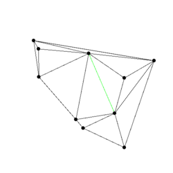
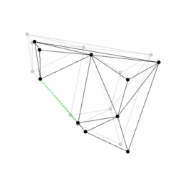
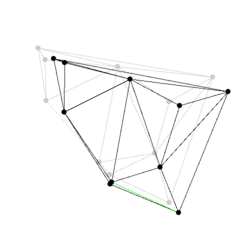
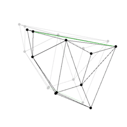
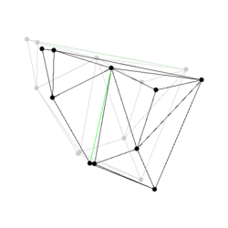
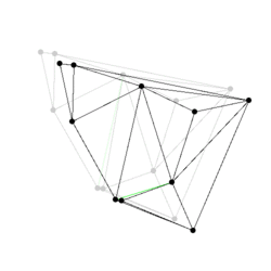
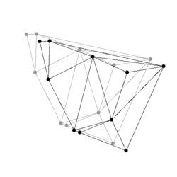
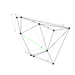
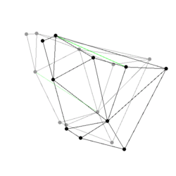
Figure:
Some events from a Delaunay triangulation kinetic data
structure: The state of the two dimensional Delaunay triangulation
immediately following the first events is shown. Green edges are ones
which were just created. The pictures are screen shots from
demo/Kinetic_data_structures/Kinetic_Delaunay_triangulation_2.cpp.
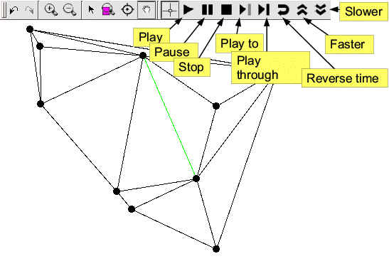
Figure 71.2: The figure shows the graphical user interface for
controlling two-dimensional kinetic data structures. It is built on
top of the Qt_widget and adds buttons to play, pause, step
through and run the simulation backwards.
71.4.4 Extending Kinetic Data Structures
Here we present a simple example that uses the
Kinetic::Sort<Traits, Visitor> kinetic data structure to compute
an arrangement of algebraic functions. It wraps the sorting data
structure and uses a visitor to monitor changes and map them to
corresponding features in the arrangement. To see an example using
this kinetic data structure read the example at
examples/Kinetic_data_structures/Kinetic_sweepline.cpp.
First we define the visitor class. An object of this type is passed to
the Kinetic::Sort<Traits, Visitor> data structure and turns
events into calls on the arrangement structure. This class has to be
defined externally since the arrangement will inherit from the sorting
structure.
template <class Arrangement>
struct Arrangement_visitor: public Kinetic::Sort_visitor_base
{
  Arrangement_visitor(Arrangement *a):p_(a){}
  template <class Vertex_handle>
  void remove_vertex(Vertex_handle a) {
    p_->erase(a);
  }
  template <class Vertex_handle>
  void create_vertex(Vertex_handle a) {
    p_->insert(a);
  }
  template <class Vertex_handle>
  void after_swap(Vertex_handle a, Vertex_handle b) {
    p_->swap(a, b);
  }
  Arrangement *p_;
};
Now we define the actual arrangement data structure.
template <class TraitsT>
class Planar_arrangement:
  public Kinetic::Sort<TraitsT,
		       Arrangement_visitor<Planar_arrangement<TraitsT> > > {
  typedef TraitsT Traits;
  typedef Planar_arrangement<TraitsT> This;
  typedef typename Kinetic::Sort<TraitsT,
				 Arrangement_visitor<This> > Sort;
  typedef Arrangement_visitor<This> Visitor;
  typedef typename Traits::Active_objects_table::Key Key;

public:
  typedef CGAL::Exact_predicates_inexact_constructions_kernel::Point_2 Approximate_point;
  typedef std::pair<int,int> Edge;
  typedef typename Sort::Vertex_handle Vertex_handle;

  // Register this KDS with the MovingObjectTable and the Simulator
  Planar_arrangement(Traits tr): Sort(tr, Visitor(this)) {}

  Approximate_point vertex(int i) const
  {
    return approx_coords_[i];
  }

  size_t vertices_size() const
  {
    return approx_coords_.size();
  }

  typedef std::vector<Edge >::const_iterator Edges_iterator;
  Edges_iterator edges_begin() const
  {
    return edges_.begin();
  }
  Edges_iterator edges_end() const
  {
    return edges_.end();
  }

  void insert(Vertex_handle k) {
    last_points_[*k]=new_point(*k);
  }

  void swap(Vertex_handle a, Vertex_handle b) {
    int swap_point= new_point(*a);
    edges_.push_back(Edge(swap_point, last_points_[*a]));
    edges_.push_back(Edge(swap_point, last_points_[*b]));
    last_points_[*a]= swap_point;
    last_points_[*b]= swap_point;
  }

  void erase(Vertex_handle a) {
    edges_.push_back(Edge(last_points_[*a], new_point(*a)));
  }

  int new_point(typename Traits::Active_objects_table::Key k) {
    double tv= CGAL::to_double(Sort::traits().simulator_handle()->current_time());
    double dv= CGAL::to_double(Sort::traits().active_objects_table_handle()->at(k).x()(tv));
    approx_coords_.push_back(Approximate_point(tv, dv));
    return approx_coords_.size()-1;
  }

  std::vector<Approximate_point > approx_coords_;
  std::map<Key, int> last_points_;
  std::vector<Edge> edges_;

};
Finally, we have to set everything up. To do this we use some special
event classes: Kinetic::Insert_event<ActiveObjectsTable> and
Kinetic::Erase_event<ActiveObjectsTable>. These are events which
can be put in the event queue which either insert a primitive into the
set of active objects or remove it. Using these, we can allow curves
in the arrangement to begin or end in arbitrary places.
typedef CGAL::Kinetic::Insert_event<Traits::Active_points_1_table> Insert_event;
typedef CGAL::Kinetic::Erase_event<Traits::Active_points_1_table> Erase_event;
do {
  NT begin, end;
  Point function;
  // initialize the function and the beginning and end somewhere
  tr.simulator_handle()->new_event(Time(begin),
			      Insert_event(function, tr.active_points_1_table_handle()));
  tr.simulator_handle()->new_event(Time(end),
				      Erase_event(Traits::Active_points_1_table::Key(num),
						  tr.active_points_1_table_handle()));
  ++num;
} while (true);