
|
CGAL 6.1.1 - 2D Generalized Barycentric Coordinates
|
Loading...
Searching...
No Matches
|
CGAL 6.1.1 - 2D Generalized Barycentric Coordinates
|
Barycentric coordinates are widely used in computer graphics and computational mechanics to determine a position of a point in the plane with respect to a triangle. These coordinates have been later generalized to support simple polygons in 2D and polyhedra in 3D.
This package offers an efficient and robust implementation of 2D generalized barycentric coordinates defined for simple polygons in the plane. If coordinates with respect to multivariate scattered points instead of a polygon are required, please refer to natural neighbor coordinates from the package 2D and Surface Function Interpolation.
In particular, this package includes an implementation of Wachspress, discrete harmonic, mean value, and harmonic coordinates, and provides some extra functions to compute barycentric coordinates with respect to segments and triangles.
Figure 108.1 Wachspress (WP), discrete harmonic (DH), mean value (MV), and harmonic (HM) coordinate functions for a convex polygon plotted with respect to the marked vertex.
Mean value and harmonic coordinates are the most generic coordinates in this package, because they allow an arbitrary simple polygon as input. Wachspress and discrete harmonic coordinates are, by definition, limited to strictly convex polygons. Segment coordinates take as input any non-degenerate segment, and triangle coordinates allow an arbitrary non-degenerate triangle.
Wachspress, discrete harmonic, mean value, and harmonic coordinates are all generalized barycentric coordinates. However, while Wachspress, discrete harmonic, and mean value coordinates can be computed analytically, harmonic coordinates cannot. They first need to be approximated over a triangulation of the interior part of the polygon. Once approximated, they can be evaluated analytically at any point inside the polygon.
For all analytic coordinates, we provide two algorithms. One has a linear time complexity, but may suffer imprecisions near the polygon boundary, while the second one is precise but has a quadratic time complexity. The user can choose the preferred algorithm by specifying a computation policy Barycentric_coordinates::Computation_policy_2.
All analytic barycentric coordinates for polygons can be computed either by instantiating a class or through one of the free functions. Harmonic coordinates can be computed only by instantiating a class that must be parameterized by a model of the concept DiscretizedDomain_2. Segment and triangle coordinates can be computed only through the free functions. For more information see the Reference Manual.
Any point in the plane may be taken as a query point. However, we do not recommend using Wachspress and discrete harmonic coordinates with query points outside the closure of a polygon, because they are not well-defined for some of these points. The same holds for harmonic coordinates, which are not defined everywhere outside the polygon. For more information see Section Edge Cases.
The output of the computation is a set of coordinate values at the given query point with respect to the polygon vertices. That means that the number of returned coordinates per query point equates the number of polygon vertices. The ordering of the coordinates is the same as the ordering of polygon vertices.
All class and function templates are parameterized by a traits class, which is a model of the concept BarycentricTraits_2. It provides all necessary geometric primitives, predicates, and constructions, which are required for the computation. All models of Kernel can be used. A polygon is provided as a range of vertices with a property map that maps a vertex from the polygon to CGAL::Point_2.
If you do not know which coordinate function best fits your application, you can address the table below for some advise.
| Coordinates | Properties | Valid domain | Closed form | Queries | Speed |
|---|---|---|---|---|---|
| Segment | All | 2D non-degenerate segments | Yes | Everywhere on the supporting line | +++ |
| Triangle | All | 2D non-degenerate triangles | Yes | Everywhere in 2D | +++ |
| Discrete harmonic | May be negative | Strongly convex polygons | Yes | Everywhere inside the polygon | ++ |
| Wachspress | All | Strongly convex polygons | Yes | Everywhere inside the polygon | ++ |
| Mean value | May be negative | Simple polygons | Yes | Everywhere in 2D | ++ |
| Harmonic | All | Simple polygons | No | Everywhere inside the polygon | + |
In order to facilitate the process of learning this package, we provide various examples with a basic usage of different barycentric components.
This example illustrates the use of the global function segment_coordinates_2(). We compute coordinates at three green points along the segment \([v_0, v_1]\) and at two blue points outside this segment but along its supporting line. The symmetry of the query points helps recognizing errors that may have occurred during construction of the example. The used Kernel is exact.
Figure 108.2 Example's point pattern.
File Barycentric_coordinates_2/segment_coordinates.cpp
In this example, we show how to use the global function triangle_coordinates_2(). We compute coordinates for three sets of points: interior (green), boundary (red), and exterior (blue). Note that some of the coordinate values for the exterior points are negative. The used Kernel is inexact.
Figure 108.3 Example's point pattern.
File Barycentric_coordinates_2/triangle_coordinates.cpp
In the following example, we generate 100 random points (green/red/black), then we take the convex hull (red/black) of this set of points as our polygon (black), and compute Wachspress coordinates at all the generated points. The used Kernel is inexact.
Figure 108.4 Example's point pattern.
File Barycentric_coordinates_2/wachspress_coordinates.cpp
In this example, we compute discrete harmonic coordinates for a set of green (interior), red (boundary), and blue (exterior) points with respect to a unit square. We also demonstrate the use of various containers, both random access and serial access, different property maps, and the ability to choose a computation policy. For points on the polygon boundary, we use the free function boundary_coordinates_2(). The used Kernel is exact.
Figure 108.5 Example's point pattern.
File Barycentric_coordinates_2/discrete_harmonic_coordinates.cpp
This is an example that illustrates how to compute mean value coordinates for a set of green points in a star-shaped polygon. We note that this type of coordinates is well-defined for such a concave polygon while Wachspress and discrete harmonic coordinates are not. However, it may yield negative coordinate values for points outside the polygon's kernel (shown in red). We speed up the computation using the linear time complexity algorithm by specifying a computation policy Barycentric_coordinates::Computation_policy_2. The used Kernel is inexact.
Figure 108.6 Example's point pattern.
File Barycentric_coordinates_2/mean_value_coordinates.cpp
This example illustrates how to discretize the interior part of the polygon and compute harmonic coordinates at the vertices of the discretized domain, which is represented by a 2D Delaunay triangulation. Once computed, harmonic coordinate functions can be evaluated at any point in the closure of the polygon. To illustrate such an evaluation, we compute the barycenter of each triangle and evaluate harmonic coordinates at this barycenter. Since harmonic coordinates can only be approximated, the used Kernel is inexact.
File Barycentric_coordinates_2/harmonic_coordinates.cpp
This is an advanced example that illustrates how to use generalized barycentric coordinates for height interpolation with applications to terrain modeling. It also shows how to use a non-default traits class with our package instead of a Kernel traits class. Suppose we know the boundary of three-dimensional piece of terrain that can be represented as a polygon with several three-dimensional vertices, where the third dimension indicates the corresponding height. The task is to propagate the height from the known sample points on the boundary to the polygon's interior. This gives an approximate estimation of the terrain's surface in this region.
Figure 108.7 A 2D polygon with 50 vertices representing a piece of terrain with convex and concave parts. The height is not shown.
In this example, we project a 3D polygon orthogonally onto the 2D plane using the class CGAL::Projection_traits_xy_3, triangulate its interior using the class Delaunay_domain_2, and compute mean value coordinates at the vertices of this triangulation with respect to the polygon vertices. Finally, we interpolate the height data from the polygon boundary to its interior using the computed coordinates and the global interpolation function from the package 2D and Surface Function Interpolation.
File Barycentric_coordinates_2/terrain_height_modeling.cpp
As a result, we get a smooth function inside the polygon that approximates the underlying terrain surface.

Figure 108.8 The interpolated data. The color bar represents the corresponding height.
This is another advanced example that shows how to use generalized barycentric coordinates in order to deform a given 2D shape into another shape as shown in the figure below. Harmonic coordinates satisfy all the properties of barycentric coordinates for complicated concave polygons and hence this is our choice to perform a shape deformation. Note that even though harmonic coordinates are guaranteed to be positive inside a polygon, they do not guarantee a bijective mapping between the source and target shapes that is the target mesh can fold-over the target polygon after the mapping (see the little fold-over in the left shoulder of the target shape).
Figure 108.9 The shape on the left is deformed into the shape on the right. The zoom shows a fold-over in the left shoulder of the target shape where the red triangle goes over the polygon boundary.
File Barycentric_coordinates_2/shape_deformation.cpp
But despite the possible fold-overs, a similar technique can be used for image warping in 2D and character articulation in 3D. For example in 2D, we first enclose an image, which we want to deform, into a simple polygon so-called cage, we then bound each image pixel to this cage using barycentric coordinates, and finally deform this cage into a new one, which also deforms the underlying image, as shown in the figure below for harmonic coordinates.
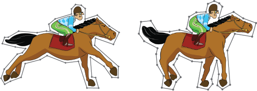
Figure 108.10 An image on the left is deformed into a new image on the right using a 2D concave polygon (grey) and harmonic coordinates computed at each image pixel with respect to the vertices of this polygon.
This is an example, where we show how a lambda expression can be used to define a model of generalized barycentric coordinates. To make this example useful, we implement affine generalized coordinates for a set of scattered points. The used Kernel is inexact.
Figure 108.11 Example's point pattern.
File Barycentric_coordinates_2/affine_coordinates.cpp
This example illustrates how to use the deprecated API of this package. The used Kernel is inexact and the used coordinates are mean value coordinates. The result is identical to the one from this example.
File Barycentric_coordinates_2/deprecated_coordinates.cpp
Segment_coordinates_2.h and Triangle_coordinates_2.h are not capitalized in the new version that is they are named segment_coordinates_2.h and triangle_coordinates_2.h.Not all presented coordinates are general enough to handle any query point in the plane, that is why we highly recommend reading this section in order to learn what can be expected from each coordinate function. If you want to get more mathematical details about each coordinate function as well as the complete history and theory behind barycentric coordinates, you should read [6]. You can also read an overview here (chapters 1 and 2).
The segment coordinate function with respect to a given segment vertex is a linear function along the supporting line of this segment that grows from zero at the opposite vertex to one at the chosen vertex (see the figure below).
Figure 108.12 The segment coordinate function with respect to the vertex \(v_0\).
Segment coordinates can be computed exactly if an exact number type is chosen. The segment itself, with respect to which we compute coordinates, must be non-degenerate. If both conditions are satisfied, then the computation never fails. However, to compute coordinates, the user must ensure that the query point lies exactly on the line \(L\) supporting the segment. Since in many applications this is not the case, and a query point may lie very close but not exactly on this line, we provide a solution to remedy this situation.
Figure 108.13 The orthogonal projection \(p'\) of the vector \(p\) (green) onto the vector \(q\) (red).
Suppose that some query point \(v\) does not lie exactly on the line \(L\), but is some distance \(d\) away as shown in the figure above. If we want to compute the segment coordinate \(b_1(v)\) with respect to the vertex \(v_1\), we first find the orthogonal projection \(p'\) of the vector \(p\) onto the vector \(q\) and then normalize it by the length of \(q\). This yields the segment coordinate \(b_1(v') = b_1(v)\) if \(v\) lies exactly on the line. The other segment coordinate \(b_0(v')\) that is equal to \(b_0(v)\) when \(v\) is on the line \(L\) is computed the same way but with the projection of the vector \(\vec{vv_1}\).
Warning: do not abuse the feature described above, because it does not yield correct segment coordinates for the point \(v\) but rather those for \(v'\). Moreover, segment coordinates for a point \(v\), which does not lie exactly on the line \(L\), do not exist. But if the non-zero distance \(d\) is due to some numerical instability when computing the location of the point \(v\) or any other problem, which causes the point to be not exactly on the line, the final segment coordinates will be, at least approximately, correct.
With inexact number types, the resulting coordinate values are correct up to the precision of the chosen type.
The triangle coordinate function with respect to a given triangle vertex is a linear function that grows from zero along the opposite edge to one at the chosen vertex (see the figure below).
Figure 108.14 The triangle coordinate function with respect to the vertex \(v_0\).
To compute the triangle coordinates of the query point \(v\), we adopt the standard simple formula
where \(A_i\) is the signed area of the sub-triangle opposite to the vertex \(i\) and \(A\) is the total area of the triangle that is \(A = A_0 + A_1 + A_2\) (see the figure below).
Figure 108.15 Notation for triangle coordinates.
These coordinates can be computed exactly if an exact number type is chosen, for any query point in the plane and with respect to any non-degenerate triangle. No special cases are handled. The computation always yields the correct result. The notion of correctness depends on the precision of the used number type. Note that for exterior points some coordinate values will be negative.
Wachspress coordinates are well-defined in the closure of any strictly convex polygon. Therefore, when using an exact number type, for any query point from the polygon's closure, these coordinates are computed exactly and no false result is expected. For exterior query points, the coordinates can also be computed but not everywhere (see below for more details). For inexact number types, the resulting precision of the computation is due to the involved algorithm and a chosen number type. In the following paragraph, we discuss two available algorithms for computing Wachspress coordinates when an inexact number type is used. The chosen algorithm is specified by a computation policy Barycentric_coordinates::Computation_policy_2.
Figure 108.16 Notation for Wachspress coordinates.
To compute Wachspress weights, we follow [2] and use the formula
with \(i = 1\dots n\) where \(n\) is the number of polygon vertices. In order to compute the coordinates, we normalize these weights,
This formula becomes unstable when approaching the boundary of the polygon ( \(\approx 1.0e-10\) and closer). To fix the problem, we modify the weights \(w_i\) as
After the above normalization, this gives us the precise algorithm to compute Wachspress coordinates but with \(O(n^2)\) performance only. The max speed \(O(n)\) algorithm uses the standard weights \(w_i\). Note that mathematically this modification does not change the coordinates. One should be cautious when using the unnormalized Wachspress weights. In that case, you must choose the \(O(n)\) type.
It is known that for strictly convex polygons the denominator's zero set of the Wachspress coordinates ( \(W^{wp} = 0~\)) is a curve, which (in many cases) lies quite far away from the polygon. More specifically, it interpolates the intersection points of the supporting lines of the polygon edges. Therefore, the computation of Wachspress coordinates outside the polygon is possible only at points that do not belong to this curve.
Figure 108.17 Zero set (red) of the Wachspress coordinates' denominator \(W^{wp}\) for a non-regular hexagon.
Warning: we do not recommend using Wachspress coordinates for exterior points!
Discrete harmonic coordinates have the same requirements as Wachspress coordinates. They are well-defined in the closure of any strictly convex polygon and, if an exact number type is chosen, they are computed exactly. However, and unlike Wachspress basis functions, these coordinates are not necessarily positive. In particular, the weight \(w_i\) is positive if and only if \(\alpha+\beta < \pi\) (see the figure below for notation). For inexact number types, the precision of the computation is due to the involved algorithm and a chosen number type. Again, we describe two algorithms to compute the coordinates when an inexact number type is used: one is of max precision and one is of max speed.
Figure 108.18 Notation for discrete harmonic coordinates.
To compute discrete harmonic weights, we follow [2] and use the formula
with \(i = 1\dots n\) where \(n\) is the number of polygon vertices. In order to compute the coordinates, we normalize these weights,
This formula becomes unstable when approaching the boundary of the polygon ( \(\approx 1.0e-10\) and closer). To fix the problem, similarly to the previous subsection, we modify the weights \(w_i\) as
After the above normalization, this yields the precise algorithm to compute discrete harmonic coordinates but with \(O(n^2)\) performance only. The max speed \(O(n)\) algorithm uses the standard weights \(w_i\). Again, mathematically this modification does not change the coordinates, one should be cautious when using the unnormalized discrete harmonic weights. In that case, you must choose the \(O(n)\) type.
Warning: as for Wachspress coordinates, we do not recommend using discrete harmonic coordinates for exterior points, because the curve \(W^{dh} = 0\) may have several components, and one of them interpolates the polygon vertices. However, if you are sure that the query point does not belong to this curve, you can compute the coordinates as shown in this example.
Unlike the previous coordinates, mean value coordinates cannot be computed exactly due to an inevitable square root operation. Although, if an exact number type is used, the default precision of the computation depends only on two CGAL functions: CGAL::to_double() and CGAL::sqrt(). It is worth saying that providing a number type that supports exact or nearly exact computation of the square root is possible, however since such types are usually impractical due to the large overhead, the conversion to a floating-point format above is always effective. On the other hand, mean value coordinates are well-defined everywhere in the plane for any simple polygon. In addition, if your traits class provides a more precise version of the square root function, the final precision of the computation with exact number types will depend only on the precision of that function.
Figure 108.19 Notation for mean value coordinates.
For these coordinates, we provide two algorithms: one is of max precision and one is of max speed. The first one works everywhere in the plane, and the precision of the computation depends only on the chosen number type, including the remarks above. This algorithm is based on the following weight formula from [4]
Since \(\bar{w}_i\) is always positive, we must append to it the proper sign \(\sigma_i\) of the signed mean value weight, which can be found efficiently (see the figures below). This weight is always positive to the left of the red piecewise linear curve, and it is negative to the right of this curve, moving in the counterclockwise direction.
Figure 108.20 Signs of the mean value weight \(w_i\) depending on the region with respect to a convex polygon \(P\) and a concave polygon \(P'\).
After the normalization of these weights as before
we obtain the max precision \(O(n^2)\) algorithm. The max speed \(O(n)\) algorithm computes the weights \(w_i\) using the pseudocode from here. These weights
are also normalized. Note that they are unstable if a query point is closer than \(\approx 1.0e-10\) to the polygon boundary, similarly to Wachspress and discrete harmonic coordinates and one should be cautious when using the unnormalized mean value weights. In that case, you must choose the \(O(n)\) type.
The harmonic coordinates are computed by solving the Laplace equation
subject to suitable Dirichlet boundary conditions. Harmonic coordinates are the only coordinates in this package, which are guaranteed to be non-negative in the closure of any simple polygon and satisfy all properties of barycentric coordinates, however such desirable properties come with the fact that these coordinates are well-defined only inside a polygon. If an exterior query point is provided, its coordinates are set to zero.
Another disadvantage of these coordinates is that they cannot be computed exactly, because harmonic coordinates do not have a simple closed-form expression and must be approximated. The common way to approximate these coordinates is by discretizing over the space of piecewise linear functions with respect to a triangulation of the polygon. The denser triangulation of the interior part of the polygon, the better approximation of the coordinates. To get a high quality approximation of the coordinates, the user should provide a rather dense partition of the polygon's interior domain that in turn leads to larger running times when computing the coordinates.
Figure 108.21 Sparse triangulation of the polygon's interior domain (left): smaller running times, lower coordinates quality; dense triangulation (right): larger running times, higher coordinates quality.
From all this follows, that any exact Kernel will be rejected and it is not possible to compute analytic harmonic weights. However, once the coordinates are computed at the vertices of the triangulation, they can be evaluated analytically at any interior query point. For evaluation, we first locate a triangle that contains the query point and then linearly interpolate harmonic coordinates defined at the vertices of this triangle to the query point with the help of triangle coordinates as
with \(i = 1\dots n\), where \(n\) is the number of polygon vertices, \(b_{0}^{tr}\), \(b_{1}^{tr}\), and \(b_{2}^{tr}\) are the triangle coordinates of the query point with respect the three vertices of the located triangle, and \(b_i^{0}\), \(b_i^{1}\), and \(b_i^{2}\) are the harmonic coordinates pre-computed at the triangle vertices.
We strive for robustness and efficiency at the same time. Efficiency is especially important. These coordinates are used in many applications where they must be computed for millions of points and, thus, the real time computation of coordinates has been made possible. In this section, we present next the computation runtimes of the implemented algorithms.
The structure of the speed test that we use to evaluate the running times consists of computing coordinate values (or weights) at >= 1 million strictly interior points with respect to a polygon (or triangle, or segment). At each iteration of the loop, we create a query point and compute its coordinates. The time presented in the log-log scale plot at the end of the section is the arithmetic mean of all trials in the loop of 10 iterations. The time presented in the plot is for analytic coordinates only since harmonic coordinates of a reasonable (application-dependent) quality are substantially slower to compute and cannot be fairly compared to the analytic coordinate functions.
The time to compute coordinates depends on many factors such as memory allocation, input kernel, output container, number of points, etc. In our tests, we used the most standard C++ and CGAL features with minimum memory allocation. Therefore, the final time presented is the average time that can be expected without deep optimization but still with efficient memory allocation. It also means that it may vary depending on the usage of the package.
To benchmark analytic coordinates, we used a MacBook Pro 2011 with 2 GHz Intel Core i7 processor (2 cores) and 8 GB 1333 MHz DDR3 memory. The installed operating system was OS X 10.9 Maverick. The resulting timings for all closed-form coordinates can be found in the figure below.
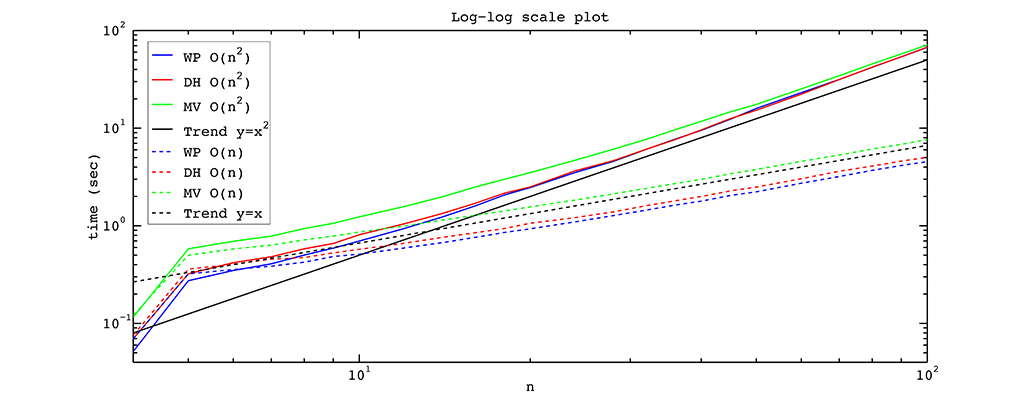
Figure 108.22 Time in seconds to compute \(n\) coordinate values for a polygon with \(n\) vertices at 1 million query points with the max speed \(O(n)\) algorithms (dashed) and the max precision \(0(n^2)\) algorithms (solid) for Wachspress (blue), discrete harmonic (red), and mean value (green) coordinates.
From the figure above we observe that the \(O(n^2)\) algorithm is as fast as the \(O(n)\) algorithm if we have a polygon with a small number of vertices. But as the number of vertices is increased, the linear algorithm outperforms the squared one, as expected. One of the reasons for this behavior is that for a small number of vertices the multiplications of \(n-2\) elements inside the \(O(n^2)\) algorithm take almost the same time as the corresponding divisions in the \(O(n)\) algorithm. For a polygon with many vertices, these multiplications are substantially slower.
To benchmark harmonic coordinates, we used a MacBook Pro 2018 with 2.2 GHz Intel Core i7 processor (6 cores) and 32 GB 2400 MHz DDR4 memory. The installed operating system was OS X 10.15 Catalina. The average time to compute harmonic coordinates in the loop of 10 iterations can be found in the tables below.
The first table shows how the time to compute the coordinates on a unit square depends on the number of triangulation vertices. We show separately the time to setup the matrix, factorize it, and solve it with respect to the four vertices of the unit square.
| Number of queries (approx.) | Setup (in seconds) | Factorize (in seconds) | Solve (in seconds) | Total (in seconds) |
|---|---|---|---|---|
| 100 | 0.000056 | 0.000099 | 0.000015 | 0.000170 |
| 500 | 0.000266 | 0.000574 | 0.000064 | 0.000904 |
| 1,000 | 0.000509 | 0.001194 | 0.000147 | 0.001850 |
| 25,000 | 0.014749 | 0.071152 | 0.008191 | 0.094092 |
| 50,000 | 0.034255 | 0.184237 | 0.018166 | 0.236658 |
| 100,000 | 0.065117 | 0.543177 | 0.044088 | 0.652382 |
| 500,000 | 0.576530 | 7.697143 | 0.310765 | 8.584438 |
| 1,000,000 | 1.295163 | 26.76945 | 0.737372 | 28.80199 |
The same results can be seen in the figure.
Figure 108.23 Time in seconds to setup (red), factorize (green), and solve (blue) for harmonic coordinate values with respect to a unit square.
The second table shows how the time to compute the coordinates for 100k queries depends on the number of the polygon vertices. We show separately the time to setup the matrix, factorize it, and solve it with respect to the \(n\) vertices of the polygon. It can be seen that, unlike in the first table, the time to factorize the matrix here stays constant.
| Number of vertices (approx.) | Setup (in seconds) | Factorize (in seconds) | Solve (in seconds) | Total (in seconds) |
|---|---|---|---|---|
| 5 | 0.083444 | 0.631823 | 0.059827 | 0.775094 |
| 10 | 0.060294 | 0.450534 | 0.094583 | 0.605411 |
| 25 | 0.062760 | 0.478683 | 0.254953 | 0.796396 |
| 50 | 0.097359 | 0.492233 | 0.539654 | 1.129246 |
| 100 | 0.129487 | 0.450771 | 1.152544 | 1.732802 |
| 500 | 0.430694 | 0.460321 | 6.620061 | 7.511076 |
| 1000 | 0.812362 | 0.480052 | 16.14239 | 17.43480 |
The same results can be seen in the figure.
Figure 108.24 Time in seconds to setup (red), factorize (green), and solve (blue) for harmonic coordinate values with respect to a polygon with \(n\) vertices at 100k query points.
While, in the first table, the most significant step is to factorize the matrix, in the second table, the slowest step is to solve for coordinates, as expected.
The package was first released in 2015 and included segment, triangle, Wachspress, discrete harmonic, and mean value coordinates. The API of that version is now deprecated but can still be used. An example of the old API can be found here. The docs of that API are also preserved and maintained here.
In 2018, this package was modified and improved by Keyu Chen and Dmitry Anisimov during the Google Summer of Code. The API was changed to the current version. In 2020, the new version was cleaned up and documented that includes:
Segment_coordinates_2 and Triangle_coordinates_2 have been removed, only the free functions are preserved;Generalized_barycentric_coordinates_2 was removed since it is not flexible enough to accommodate all types of 2D barycentric coordinates;Wachspress_2, Discrete harmonic_2, and Mean_value_2 have been renamed and modified so that they can be used now on their own without the class Generalized_barycentric_coordinates_2;The authors wish to thank Teseo Schneider and Randolf Schaerfig for helpful comments and discussions. We also appreciate the great effort invested in this package by our reviewers Andreas Fabri, Sébastien Loriot, and Efi Fogel.