
|
CGAL 6.2 - Triangulated Surface Mesh Approximation
|
Loading...
Searching...
No Matches
|
CGAL 6.2 - Triangulated Surface Mesh Approximation
|
This package implements the Variational Shape Approximation [1] (VSA) method to approximate an input surface mesh by a simpler surface triangle mesh. The input of the algorithm must be:
The output is a triangle soup and can be built into a polygon surface mesh.
Given an input surface triangle mesh, VSA leverages a discrete clustering algorithm to approximate it by a set of local simple shapes referred to as proxies. Each cluster is represented as a connected set of triangles of the input mesh, and the output mesh is constructed by generating a surface triangle mesh which approximates the clusters. The approximation error is one-sided, defined between the clusters and their associated proxies. Two error metrics ( \( \mathcal{L}^2 \), \( \mathcal{L}^{2,1} \)) for planar proxies are provided via the classes CGAL::Surface_mesh_approximation::L2_metric_plane_proxy and CGAL::Surface_mesh_approximation::L21_metric_plane_proxy, and the algorithm design is generic to other user-defined metrics. The current proxies are planes or vectors, however the algorithm design is generic for future extensions to non-planar proxies [4][3]. The default \( \mathcal{L}^{2,1} \) metric is recommended in terms of computation and visual perception [1]. A brief background about Proxy and ErrorMetric is provided in Section Background.
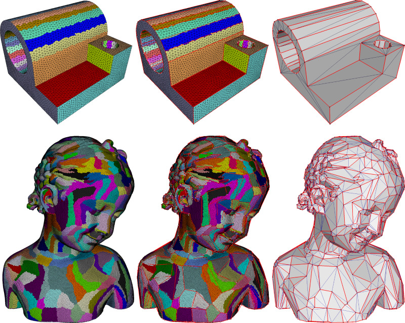
Figure 87.1 Variational shape approximation on two models with the \( \mathcal{L}^{2,1} \) error metric and planar proxies. From left to right: partition of the input surface triangle mesh, anchor vertices and edges, and output triangle mesh. The partition is optimized via discrete clustering of the input triangles, so as to minimize the approximation error from the clusters to the planar proxies (not shown).
This package offers both the approximation and mesh construction functionalities, through the free function CGAL::Surface_mesh_approximation::approximate_triangle_mesh() which runs a fully automated version of the algorithm: Example: Surface_mesh_approximation/vsa_simple_approximation_example.cpp
A class interface is also provided for advanced users, in which a series of pliant operators offer interactive capabilities during clustering and customization in terms of error and proxies.
The package contains 3 main components: approximation algorithm, pliant operators and meshing as shown in Figure 87.2.
Figure 87.2 From left to right are 3 components of the approximation package: approximation algorithm (left), optional pliant operations (middle) and meshing (right).
The left part of Figure 87.2 depicts the workflow of the approximation algorithm.
Figure 87.3 depicts several Lloyd [2] clustering iterations on the plane-sphere model with planar proxies and the \( \mathcal{L}^{2,1} \) metric. We plot the fitting error against each iteration. After 8 iterations, the error barely changes. Based on this observation, we consider that the clustering converges if the error change between the current and previous iteration is lower than a user-specified threshold (indicated by two green dash lines).
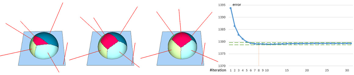
Figure 87.3 Discrete Lloyd iterations on the plane-sphere model with planar proxies and the \( \mathcal{L}^{2,1} \) metric: (left) random seeding of 6 proxies; (center) after one iteration; (right) after 8 iterations, the regions settle. The red lines depict the proxy normals drawn at the seed faces.
Each proxy is always associated to a seed triangle face in the input surface mesh. While the proxies may be viewed as centers (or best representative) in a geometric error sense, the seed of each proxy is used as the starting point in the clustering process. Seeding is the processing of deciding how to select a seed face where a new proxy/partition can be initialized from.
To start the clustering iterations, we need an initial set of proxies. The default (hierarchical) approach generates one proxy per connected component, seeded at arbitrarily chosen faces. It then adds more proxies in batches, in order to drive the error down. After each batch of proxies added, it performs several inner clustering iterations, which is referred to as relaxation in the seeding step.
Assuming a clustering partition of \(n\) regions with errors \( \{E_k\}_{k=1\cdots n} \), and we wish to add \(m\) proxies. We provide 3 different seeding methods:
\[ N_k = \lfloor E_k / E_{avg} + 0.5 \rfloor, \]
and the remaining error is added to the next proxy error in order to keep the total error unchanged:\[ E'_{k+1} = (E_k - N_k * E_{avg}) + E_{k+1}. \]
Figure 87.4 depicts different seeding methods. Random initialization randomly selects a set of input triangle faces as proxy seeds. While it is very fast, the subsequent clustering process can be entrapped in a bad local minimum, especially on shapes with regions surrounded by sharp creases (left closeup). Incremental initialization adds the proxies one by one at the most distorted region. It can thus be slow due to the large number of interleaved relaxation iterations. Hierarchical initialization (selected by default) repeatedly doubles the number of proxies in a hierarchical refinement sequence, so as to generate clustering regions with evenly distributed fitting errors. Time consumption is typically in-between the former two. Statistics and comparisons are available in Section Performances.
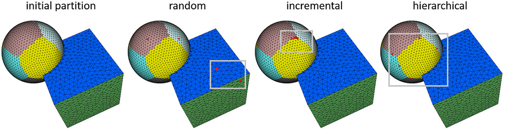
Figure 87.4 Different seeding methods on the sphere-cube model. From left to right: initial partition ( \( \mathcal{L}^{2,1} \) metrics and 20 proxies), add 5 proxy seeds (red faces) with random, incremental and hierarchical methods respectively.
To determine when to stop adding more proxies, we can specify either the maximum number of proxies required to approximate the geometry or the minimum error drop percentage with respect to the very first partition. More specifically, we can decide:
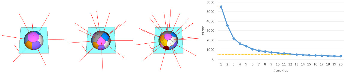
Figure 87.5 Using different number of proxies to approximate the plane-sphere model. From left to right: 8, 14, 20 proxies. We plot right the error against the number of proxies.
For interactive use, the approach can yield better approximations of the geometry via adding/removing proxies and tunneling out of local minima via additional operations:
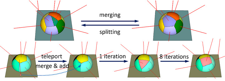
Figure 87.6 Operations on the sphere-cube union model. Upper row: merging (9 proxies) and the reverse bisection splitting (10 partitions) on the confined region. Lower row: one teleportation operation of merging and adding a face seed, the sphere is approximated with one more proxy.
As depicted in Figure 87.6, teleportation provides a means to relocate a local minimum region entrapped in the planar part (left) to the most needed regions on the sphere (right). In Class Interface, the class interface is used to control the approximation process through the aforementioned operations.
This package implements the meshing algorithm described in [1] by generating a triangle mesh approximation of the clustering partition. The meshing algorithm has two major steps:
A vertex is selected as a basic anchor if it is:
Walking along the boundary of a proxy region (counterclockwise), a chord is a sequence of halfedges connecting two anchors. One cluster boundary cycle may consist of several chords. A connected region with holes may yield several boundary cycles (Figure 87.6, planar part before teleportation).
In order to approximate complex boundaries well, more anchors are generated by recursive chord subdivision (Figure 87.7). An anchor \( \mathbf{c} \) is added at the furthest vertex of a chord \( (\mathbf{a}, \mathbf{b}) \), split it into \( (\mathbf{a}, \mathbf{c}) \) and \( (\mathbf{c}, \mathbf{b}) \), if the distance \( d = \Vert \mathbf{c} , (\mathbf{a}, \mathbf{b}) \Vert \) is beyond certain threshold. To make \( d \) independent to the scale of the input:
\[ d = d / input\_mesh\_average\_edge\_length. \]
Optionally, \( d \) can be measured as the ratio of the chord length:
\[ d = d / \Vert(\mathbf{a}, \mathbf{b})\Vert. \]
Also, we can add a dihedral angle weight \( sin(\mathbf{N}_i,\mathbf{N}_j) \) to the distance measurement, where \( \mathbf{N}_i,\mathbf{N}_j \) are the normals of the proxies separated by the chord \( (\mathbf{a}, \mathbf{b}) \). If the angle between proxy \( P_i \) and \( P_j \) is rather small, then a coarse approximation will do as it does not add geometric information on the shape. Trivial chords (made of a single edge) are not subdivided. In case of circular chords, additional anchors may be added to maintain the topology, as detailed in Section Additional Anchors.
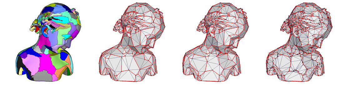
Figure 87.7 Varying the chord error. From left to right: clustering partition, and meshing with decreasing absolute chord error 5, 3 and 1 without dihedral angle weight. The boundaries of the partition (red lines) are approximated with increasing accuracy.
For a boundary cycle without any anchor such as the hole depicted Figure 87.6, we first add a starting anchor to the boundary. We then subdivide this circular chord to ensure that every boundary cycle has at least 2 anchors (i.e., every chord is connecting 2 different anchors, Figure 87.8). Finally, we add additional anchors to ensure that at least three anchor vertices are generated on every boundary cycle.
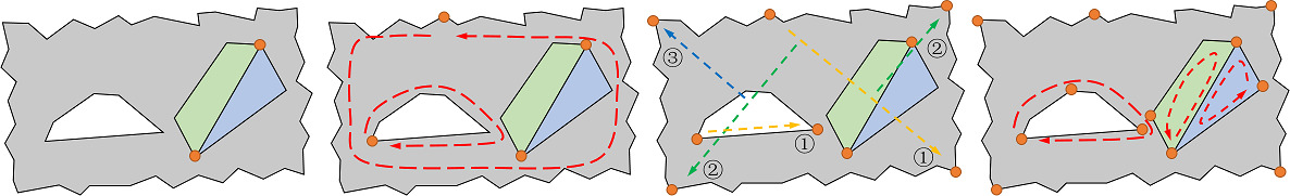
Figure 87.8 Adding anchors. From left to right: starting from a partition (grey) with a hole (white) and two encircled regions (green and blue), we add a starting anchor (orange disk) to the boundary cycle (red dash line) without any anchor (2nd), subdivide the circular chord (3rd, the number indicates the level of recursion) and add anchors to the boundary cycle with less than 2 anchors (4th, red dash lines).
With the anchors defined, their chord connection graph forms a general polygon mesh. Because of non-flat, concave polygon or polygons with holes, we need to triangulate this initial polygon mesh. The triangulation is generated by computing a discrete variant of a constrained 2D Delaunay triangulation, where distances are measured on the input triangle mesh.
The first image of Figure 87.9 depicts how the Delaunay triangulation of set of points (colored disks) is deduced from its dual Voronoi diagram (colored regions separated by blue lines) by connecting the points indicated by the vertices (red circles) where 3 Voronoi cells meet. In an analogous manner, we construct discrete Voronoi cells from which the triangulation is extracted.
In a first step, we start a flooding of the interior of the region, coloring the vertices according to their closest anchor vertex. We then only flood the boundary of a region so that every vertex on it is colored depending on the closest anchor vertex. This enforces the constrained edges by forcing the boundary to be in it.
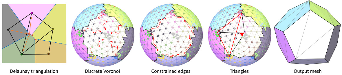
Figure 87.9 Discrete constrained triangulation on a sphere model. The triangulation process first floods the inner vertices (red arrows, 2nd) to simulate the Voronoi diagram. It then constructs constrained edges between anchor vertices, by flooding along the boundary edges (red arrows, 3rd). Finally, triangles (red hollow triangle, 4th) are formed by connecting the source anchors (black arrows, 4th) of the faces where 3 Voronoi cells meet (red solid triangle, 4th).
After each clustering region is triangulated, the final anchor positions are recomputed by averaging the projections of an anchor on its incident proxies.
In Figure 87.10, the bear model is approximated through \( \mathcal{L}^{2,1} \) metric and the final number of proxies is determined by monitoring the error drop. The anchor points (black) are attached to the corresponding vertex on the mesh (white). The red lines connecting the anchor points approximate the boundary of each region.
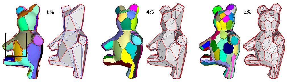
Figure 87.10 Meshing the bear model with decreasing target error drop. From left to right, the target error drop are 6%, 4% and 2% to the initial error respectively, the output mesh densifies. Notice the boundary subdivision in the black rectangle area.
As there is no guarantee that the output mesh is 2-manifold and oriented, the main input is an indexed triangle set. We can use Polygon Soups to build the triangle soup into a valid polygon mesh.
This package can be used with any class model of the concept FaceListGraph described in CGAL and the Boost Graph Library.
Free function with Named Parameters options.
CGAL::Surface_mesh_approximation::approximate_triangle_mesh(): given a triangle mesh, approximate the geometry with default \( \mathcal{L}^{2,1} \) metric.Class interface:
CGAL::Variational_shape_approximation: allowing more customization of the proxy, metric and approximation process. As shown in Figure 87.2, typical calling order of the approximation and meshing process is:
One thing to note is that some parameters depend heavily on the input, like the number of proxies. Although we can approximate a geometry with any number of proxies regardless of the quality, it is not recommended to use all the defaults without any consideration of the input.
The following example calls the free function CGAL::Surface_mesh_approximation::approximate_triangle_mesh() on the input triangle mesh with default CGAL::Surface_mesh_approximation::L21_metric_plane_proxy.
Example: Surface_mesh_approximation/vsa_approximation_example.cpp
The function parameters are provided through Named Parameters. Setting the non-default parameter values requires calling the functions with the required parameters, connected by a dot and in an arbitrary order. The following example shows a different configuration of parameters and retrieves the indexed face proxy map and the proxies:
Example: Surface_mesh_approximation/vsa_approximation_2_example.cpp
The face proxy index map and the output proxies provide a means to access the partition and the proxy parameters as illustrated by Figure 87.3.
The free function can be used for retrieving the segmentation via proxy ids output into the proxy output iterator:
Example: Surface_mesh_approximation/vsa_segmentation_example.cpp
The class interface CGAL::Variational_shape_approximation offers a flexible means to control of the algorithm. The following example uses the CGAL::Surface_mesh_approximation::L2_metric_plane_proxy to approximate the shape.
Example: Surface_mesh_approximation/vsa_class_interface_example.cpp
Figure 87.11 Comparison of different error metrics on the bear model, with 200 proxies and hierarchical seeding. From left to right: \( \mathcal{L}^{2,1} \) metric, \( \mathcal{L}^2 \) metric and custom compact metric.
The following example defines a point-wise proxy to yield an isotropic approximation. The output mesh is depicted in Figure 87.11.
Example: Surface_mesh_approximation/vsa_isotropic_metric_example.cpp
We provide some performance comparisons with the free function API CGAL::Surface_mesh_approximation::approximate_triangle_mesh. Timings are recorded on a PC running Windows10 X64 with an Intel Xeon E5-1620 clocked at 3.70 GHz with 32GB of RAM. The program has been optimized with the O2 option with Visual Studio 2015. By default the kernel used is Exact_predicates_inexact_constructions_kernel (EPICK).
Runtime in seconds with target number of proxies of different seeding method:
| Model | #Triangles | #Proxies | Random | Incremental | Hierarchical |
|---|---|---|---|---|---|
| plane-sphere | 6,826 | 20 | 0 | 0.87 | 0.17 |
| bear | 20,188 | 200 | 0 | 36.749 | 1.194 |
| masque | 62,467 | 200 | 0.002 | 133.901 | 4.308 |
Runtime in seconds with target error drop of different seeding method. The benchmark is running on the bear model with 20,188 faces. Each column records the time and the resulting number of proxies:
| Target Error Drop | Random | Incremental | Hierarchical |
|---|---|---|---|
| 0.06 | 1.03/64 | 9.053/53 | 1.017/64 |
| 0.04 | 1.207/128 | 15.422/88 | 1.2/128 |
| 0.02 | 1.415/256 | 35.171/192 | 1.428/256 |
Runtime of the 3 phases of the algorithm in seconds: seeding, clustering iteration and meshing. The seeding method is hierarchical with target number of proxies.
| Model | #Triangles | #Proxies | #Iterations | Seeding | Clustering | Meshing | Total |
|---|---|---|---|---|---|---|---|
| plane-sphere | 6,826 | 20 | 20 | 0.17 | 0.228 | 0.044 | 0.442 |
| bear | 20,188 | 200 | 20 | 1.194 | 0.784 | 0.128 | 2.006 |
| masque | 62,467 | 200 | 20 | 4.308 | 2.974 | 0.349 | 7.631 |
The VSA method has two key geometric concepts:
Given an error metric \( E \), a desired number of \( k \) proxies, and an input surface \( S \), we denote by optimal shape proxies a set \( P \) of proxies \( P_i \) associated to the regions \( R_i\) of a partition \( \mathcal{R} \) of \( S \) that minimizes the total fitting error [1] :
\[ E(\mathcal{R}, P) = \sum_{i = 1..k} E(\mathcal{R}_i, P_i). \]
By casting the approximation problem into an optimal discrete clustering one, the algorithm leverages the effective Lloyd algorithm [1] to drive the total error down iteratively. More specifically, during each iteration two different steps are conducted, for the \( m \)th iteration:
For a sequence of iterations with the fitting error \( \{ E^1, \cdots, E^m \} \), the iteration is repeated until one of the stopping criteria is met:
Intuitively, each region \( \mathcal{R}_i \) of a partition \( \mathcal{R} \) can be summarily represented to first order as an "average" point \( X_i \) and an "average" normal \( N_i \). We denote such local representative pair \( P_i = (X_i, N_i) \), a planar proxy of the associated region.
Defining an appropriate error metric is the key ingredient for the algorithm. The \( \mathcal{L}^2 \) metric is defined as:
\[ \mathcal{L}^2(\mathcal{R}_i, P_i) = \iint_{x \in \mathcal{R}_i}\Vert x - \Pi_i(x)\Vert^2 dx. \]
where \( \Pi_i(\cdot) \) denotes the orthogonal projection of the argument onto the proxy plane passing through \( X_i \) and normal to \( N_i \). The \( \mathcal{L}^2 \) metric tries to match the input shape through approximation of the geometric position.
In the original paper [1] the author proposed the \( \mathcal{L}^{2,1} \) metrics, arguing that the normals are important to the visual interpretation of the shape. The \( \mathcal{L}^{2,1} \) is defined as:
\[ \mathcal{L}^{2,1}(\mathcal{R}_i, P_i) = \iint_{x \in \mathcal{R}_i}\Vert \mathbf{n}(x) - \mathbf{n}_i\Vert^2 dx. \]
The \( \mathcal{L}^{2,1} \) is numerically superior to \( \mathcal{L}^2 \) in several ways:
This package is the result of the work of Lingjie Zhu during the 2017 season of the Google Summer of Code, mentored by Pierre Alliez. The code is based on an initial research code written by Pierre Alliez at Inria in 2003, for a paper published at the ACM SIGGRAPH conference in 2004, co-authored by David Cohen-Steiner, Pierre Alliez and Mathieu Desbrun [1].