

|
CGAL 4.5.2 - 2D and Surface Function Interpolation
|
|
CGAL 4.5.2 - 2D and Surface Function Interpolation
|
This chapter describes CGAL's interpolation package which implements natural neighbor coordinate functions as well as different methods for scattered data interpolation most of which are based on natural neighbor coordinates. The functions for computing natural neighbor coordinates in Euclidean space are described in Section Natural Neighbor Coordinates, the functions concerning the coordinate and neighbor computation on surfaces are discussed in Section Surface Natural Neighbor Coordinates and Surface Neighbors. In Section Interpolation Methods, we describe the different interpolation functions.
Scattered data interpolation solves the following problem: given measures of a function on a set of discrete data points, the task is to interpolate this function on an arbitrary query point. More formally, let \( \mathcal{P}=\{\mathbf{p_1},\ldots ,\mathbf{p_n}\}\) be a set of \( n\) points in \( \mathbb{R}^2\) or \( \mathbb{R}^3\) and \( \Phi\) be a scalar function defined on the convex hull of \( \mathcal{P}\). We assume that the function values are known at the points of \( \mathcal{P}\), i.e. to each \( \mathbf{p_i} \in \mathcal{P}\), we associate \( z_i = \Phi(\mathbf{p_i})\). Sometimes, the gradient of \( \Phi\) is also known at \( \mathbf{p_i}\). It is denoted \( \mathbf{g_i}= \nabla \Phi(\mathbf{p_i})\). The interpolation is carried out for an arbitrary query point \( \mathbf{x}\) on the convex hull of \( \mathcal{P}\).
Natural neighbor interpolation has been introduced by Sibson [9] to interpolate multivariate scattered data. Given a set of data points \( \mathcal{P}\), the natural neighbor coordinates associated to \( \mathcal{P}\) are defined from the Voronoi diagram of \( \mathcal{P}\). When simulating the insertion of a query point \( \mathbf{x}\) into the Voronoi diagram of \( \mathcal{P}\), the potential Voronoi cell of \( \mathbf{x}\) "steals" some parts from the existing cells.
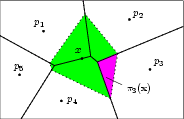
Let \( \pi(\mathbf{x})\) denote the volume of the potential Voronoi cell of \( \mathbf{x}\) and \( \pi_i(\mathbf{x})\) denote the volume of the sub-cell that would be stolen from the cell of \( \mathbf{p_i}\) by the cell of \( \mathbf{x}\). The natural neighbor coordinate of \( \mathbf{x}\) with respect to the data point \( \mathbf{p_i}\in \mathcal{P}\) is defined by
\[ \lambda_i(\mathbf{x}) = \frac{\pi_i(\mathbf{x})}{\pi(\mathbf{x})}. \]
A two-dimensional example is depicted in Figure 70.1.
Various papers ([8], [4], [7], [3], [6]) show that the natural neighbor coordinates have the following properties:
For the case where the query point x is located on the envelope of the convex hull of \( \mathcal{P}\), the potential Voronoi cell of x becomes infinite and :
\( \pi(\mathbf{x}) = \infty\)
\( \lambda_i(\mathbf{x}) = 0 \) for all data point \( \mathbf{p_i}\) of \( \mathcal{P}\) except for the two endpoints, let's say \( \mathbf{p}\) and \( \mathbf{q}\) ,of the edge where x lies.
The natural neighbor coordinate of \( \mathbf{x}\) with respect to these endpoints \( \mathbf{p}\) and \( \mathbf{q}\) will be :
\( \lambda_p(\mathbf{x}) = \frac{\|\mathbf{x} - \mathbf{q}\| }{ \|\mathbf{q} - \mathbf{p}\|} \)
\( \lambda_q(\mathbf{x}) = \frac{\|\mathbf{x} - \mathbf{p}\| }{ \|\mathbf{q} - \mathbf{p}\|} \)
Furthermore, Piper [7] shows that the coordinate functions are continuous in the convex hull of \( \mathcal{P}\) and continuously differentiable except on the data points \( \mathcal{P}\).
The interpolation package of CGAL provides functions to compute natural neighbor coordinates for \( 2D\) and \( 3D\) points with respect to Voronoi diagrams as well as with respect to power diagrams (only \( 2D\)), i.e. for weighted points. Refer to the reference pages natural_neighbor_coordinates_2(), sibson_natural_neighbor_coordinates_3() laplace_natural_neighbor_coordinates_3() and regular_neighbor_coordinates_2().
In addition, the package provides functions to compute natural neighbor coordinates on well sampled point set surfaces. See Section Surface Natural Neighbor Coordinates and Surface Neighbors and the reference page surface_neighbor_coordinates_3() for further information.
Given a Delaunay triangulation or a Regular triangulation, the vertices in conflict with the query point are determined. The areas \( \pi_i(\mathbf{x})\) are computed by triangulating the Voronoi sub-cells. The normalization factor \( \pi(\mathbf{x})\) is also returned. If the query point is already located and/or the boundary edges of the conflict zone are already determined, alternative functions allow to avoid the re-computation.
The signature of all coordinate computation functions is about the same.
File Interpolation/nn_coordinates_2.cpp
For regular neighbor coordinates, it is sufficient to replace the name of the function and the type of triangulation passed as parameter. A special traits class is needed.
File Interpolation/rn_coordinates_2.cpp
For surface neighbor coordinates, the surface normal at the query point must be provided, see Section Surface Natural Neighbor Coordinates and Surface Neighbors.
This section introduces the functions to compute natural neighbor coordinates and surface neighbors associated to a set of sample points issued from a surface \( \mathcal{S}\) and given a query point \( \mathbf{x}\) on \( \mathcal{S}\). We suppose that \( \mathcal{S}\) is a closed and compact surface of \( \mathbb{R}^3\), and let \( \mathcal{P}= \{\mathbf{p_1}, \ldots,\mathbf{p_n}\}\) be an \( \epsilon\)-sample of \( \mathcal{S}\) (refer to Amenta and Bern [1]). The concepts are based on the definition of Boissonnat and Flötotto [2], [5]. Both references contain a thorough description of the requirements and the mathematical properties.
Two observations lead to the definition of surface neighbors and surface neighbor coordinates: First, it is clear that the tangent plane \( \mathcal{T}_x\) of the surface \( \mathcal{S}\) at the point \( \mathbf{x} \in \mathcal{S}\) approximates \( \mathcal{S}\) in the neighborhood of \( \mathbf{x}\). It has been shown in [2] that, if the surface \( \mathcal{S}\) is well sampled with respect to the curvature and the local thickness of \( \mathcal{S}\), i.e. it is an \( \epsilon\)-sample, the intersection of the tangent plane \( \mathcal{T}_x\) with the Voronoi cell of \( \mathbf{x}\) in the Voronoi diagram of \( \mathcal{P} \cup \{\mathbf{x}\}\) has a small diameter. Consequently, inside this Voronoi cell, the tangent plane \( \mathcal{T}_x\) is a reasonable approximation of \( \mathcal{S}\). Furthermore, the second observation allows to compute this intersection diagram easily: one can show using Pythagoras' Theorem that the intersection of a three-dimensional Voronoi diagram with a plane \( \mathcal{H}\) is a two-dimensional power diagram. The points defining the power diagram are the projections of the points in \( \mathcal{P}\) onto \( \mathcal{H}\), each point weighted with its negative square distance to \( \mathcal{H}\). Algorithms for the computation of power diagrams via the dual regular triangulation are well known and for example provided by CGAL in the class Regular_triangulation_2<Gt, Tds>.
In CGAL, the regular triangulation dual to the intersection of a \( 3D\) Voronoi diagram with a plane \( \mathcal{H}\) can be computed by instantiating the Regular_triangulation_2<Gt, Tds> class with the traits class Voronoi_intersection_2_traits_3<K>. This traits class contains a point and a vector as class member which define the plane \( \mathcal{H}\). All predicates and constructions used by Regular_triangulation_2<Gt, Tds> are replaced by the corresponding operators on three-dimensional points. For example, the power test predicate (which takes three weighted \( 2D\) points \( p'\), \( q'\), \( r'\) of the regular triangulation and tests the power distance of a fourth point \( t'\) with respect to the power circle orthogonal to \( p\), \( q\), \( r\)) is replaced by a Side_of_plane_centered_sphere_2_3 predicate that tests the position of a \( 3D\) point \( t\) with respect to the sphere centered on the plane \( \mathcal{H}\) passing through the \( 3D\) points \( p\), \( q\), \( r\). This approach allows to avoid the explicit constructions of the projected points and the weights which are very prone to rounding errors.
The computation of natural neighbor coordinates on surfaces is based upon the computation of regular neighbor coordinates with respect to the regular triangulation that is dual to \( {\rm Vor}(\mathcal{P}) \cap \mathcal{T}_x\), the intersection of \( \mathcal{T}_x\) and the Voronoi diagram of \( \mathcal{P}\), via the function regular_neighbor_coordinates_2().
Of course, we might introduce all data points \( \mathcal{P}\) into this regular triangulation. However, this is not necessary because we are only interested in the cell of \( \mathbf{x}\). It is sufficient to guarantee that all surface neighbors of the query point \( \mathbf{x}\) are among the input points that are passed as argument to the function. The sample points \( \mathcal{P}\) can be filtered for example by distance, e.g. using range search or \( k\)-nearest neighbor queries, or with the help of the \( 3D\) Delaunay triangulation since the surface neighbors are necessarily a subset of the natural neighbors of the query point in this triangulation. CGAL provides a function that encapsulates the filtering based on the \( 3D\) Delaunay triangulation. For input points filtered by distance, functions are provided that indicate whether or not points that lie outside the input range (i.e. points that are further from \( \mathbf{x}\) than the furthest input point) can still influence the result. This allows to iteratively enlarge the set of input points until the range is sufficient to certify the result.
The surface neighbors of the query point are its neighbors in the regular triangulation that is dual to \( {\rm Vor}(\mathcal{P}) \cap \mathcal{T}_x\), the intersection of \( \mathcal{T}_x\) and the Voronoi diagram of \( \mathcal{P}\). As for surface neighbor coordinates, this regular triangulation is computed and the same kind of filtering of the data points as well as the certification described above is provided.
File Interpolation/surface_neighbor_coordinates_3.cpp
Sibson [9] defines a very simple interpolant that re-produces linear functions exactly. The interpolation of \( \Phi(\mathbf{x})\) is given as the linear combination of the neighbors' function values weighted by the coordinates:
\[ Z^0(\mathbf{x}) = \ccSum{i}{}{ \lambda_i(\mathbf{x}) z_i}. \]
Indeed, if \( z_i=a + \mathbf{b}^t \mathbf{p_i}\) for all natural neighbors of \( \mathbf{x}\), we have
\[ Z^0(\mathbf{x}) = \ccSum{i}{}{ \lambda_i(\mathbf{x}) (a + \mathbf{b}^t\mathbf{p_i})} = a+\mathbf{b}^t \mathbf{x} \]
by the barycentric coordinate property. The first example in Subsection Example for Linear Interpolation shows how the function is called.
In [9], Sibson describes a second interpolation method that relies also on the function gradient \( \mathbf{g_i}\) for all \( \mathbf{p_i} \in \mathcal{P}\). It is \( C^1\) continuous with gradient \( \mathbf{g_i}\) at \( \mathbf{p_i}\). Spherical quadrics of the form \( \Phi(\mathbf{x}) =a + \mathbf{b}^t \mathbf{x} +\gamma\ \mathbf{x}^t\mathbf{x}\) are reproduced exactly. The proof relies on the barycentric coordinate property of the natural neighbor coordinates and assumes that the gradient of \( \Phi\) at the data points is known or approximated from the function values as described in [9] (see Section Gradient Fitting).
Sibson's \( Z^1\) interpolant is a combination of the linear interpolant \( Z^0\) and an interpolant \( \xi\) which is the weighted sum of the first degree functions
\[ \xi_i(\mathbf{x}) = z_i +\mathbf{g_i}^t(\mathbf{x}-\mathbf{p_i}),\qquad \xi(\mathbf{x})= \frac{\ccSum{i}{}{ \frac{\lambda_i(\mathbf{x})} {\|\mathbf{x}-\mathbf{p_i}\|}\xi_i(\mathbf{x}) } }{\ccSum{i}{}{ \frac{\lambda_i(\mathbf{x})}{\|\mathbf{x}-\mathbf{p_i}\|}}}. \]
Sibson observed that the combination of \( Z^0\) and \( \xi\) reconstructs exactly a spherical quadric if they are mixed as follows:
\[ Z^1(\mathbf{x}) = \frac{\alpha(\mathbf{x}) Z^0(\mathbf{x}) + \beta(\mathbf{x}) \xi(\mathbf{x})}{\alpha(\mathbf{x}) + \beta(\mathbf{x})} \mbox{ where } \alpha(\mathbf{x}) = \frac{\ccSum{i}{}{ \lambda_i(\mathbf{x}) \frac{\|\mathbf{x} - \mathbf{p_i}\|^2}{f(\|\mathbf{x} - \mathbf{p_i}\|)}}}{\ccSum{i}{}{ \frac{\lambda_i(\mathbf{x})} {f(\|\mathbf{x} - \mathbf{p_i}\|)}}} \mbox{ and } \beta(\mathbf{x})= \ccSum{i}{}{ \lambda_i(\mathbf{x}) \|\mathbf{x} - \mathbf{p_i}\|^2}, \]
where in Sibson's original work, \( f(\|\mathbf{x} - \mathbf{p_i}\|) = \|\mathbf{x} - \mathbf{p_i}\|\).
CGAL contains a second implementation with \( f(\|\mathbf{x} - \mathbf{p_i}\|) = \|\mathbf{x} - \mathbf{p_i}\|^2\) which is less demanding on the number type because it avoids the square-root computation needed to compute the distance \( \|\mathbf{x} - \mathbf{p_i}\|\). The theoretical guarantees are the same (see [5]). Simply, the smaller the slope of \( f\) around \( f(0)\), the faster the interpolant approaches \( \xi_i\) as \( \mathbf{x} \rightarrow \mathbf{p_i}\).
Farin [4] extended Sibson's work and realizes a \( C^1\) continuous interpolant by embedding natural neighbor coordinates in the Bernstein-Bézier representation of a cubic simplex. If the gradient of \( \Phi\) at the data points is known, this interpolant reproduces quadratic functions exactly. The function gradient can be approximated from the function values by Sibson's method [9] (see Section Gradient Fitting) which is exact only for spherical quadrics.
Knowing the gradient \( \mathbf{g_i}\) for all \( \mathbf{p_i} \in \mathcal{P}\), we formulate a very simple interpolant that reproduces exactly quadratic functions. This interpolant is not \( C^1\) continuous in general. It is defined as follows:
\[ I^1(\mathbf{x}) = \ccSum{i}{}{ \lambda_i(\mathbf{x}) (z_i + \frac{1}{2} \mathbf{g_i}^t (\mathbf{x} - \mathbf{p_i}))} \]
Sibson describes a method to approximate the gradient of the function \( f\) from the function values on the data sites. For the data point \( \mathbf{p_i}\), we determine
\[ \mathbf{g_i} = \min_{\mathbf{g}} \ccSum{j}{}{ \frac{\lambda_j(\mathbf{p_i})}{\|\mathbf{p_i} - \mathbf{p_j}\|^2} \left( z_j - (z_i + \mathbf{g}^t (\mathbf{p_j} -\mathbf{p_i})) \right)}, \]
where \( \lambda_j(\mathbf{p_i})\) is the natural neighbor coordinate of \( \mathbf{p_i}\) with respect to \( \mathbf{p_i}\) associated to \( \mathcal{P} \setminus \{\mathbf{p_i}\}\). For spherical quadrics, the result is exact.
CGAL provides functions to approximate the gradients of all data points that are inside the convex hull. There is one function for each type of natural neighbor coordinate (i.e. natural_neighbor_coordinates_2(), regular_neighbor_coordinates_2()).
File Interpolation/linear_interpolation_2.cpp
File Interpolation/sibson_interpolation_2.cpp
An additional example in the distribution compares numerically the errors of the different interpolation functions with respect to a known function. It is distributed in the examples directory.
 1.8.4
1.8.4