

|
CGAL 5.5 - dD Spatial Searching
|
|
CGAL 5.5 - dD Spatial Searching
|
The spatial searching package implements exact and approximate distance browsing by providing implementations of algorithms supporting
both nearest and furthest neighbor searching
both exact and approximate searching
(approximate) range searching
(approximate) k-nearest and k-furthest neighbor searching
(approximate) incremental nearest and incremental furthest neighbor searching
query items representing points and spatial objects.
In these searching problems a set P of data points in d-dimensional space is given. The points can be represented by Cartesian coordinates or homogeneous coordinates. These points are preprocessed into a tree data structure, so that given any query item q the points of P can be browsed efficiently. The approximate spatial searching package is designed for data sets that are small enough to store the search structure in main memory (in contrast to approaches from databases that assume that the data reside in secondary storage).
Spatial searching supports browsing through a collection of d-dimensional spatial objects stored in a spatial data structure on the basis of their distances to a query object. The query object may be a point or an arbitrary spatial object, e.g, a d-dimensional sphere. The objects in the spatial data structure are d-dimensional points.
Often the number of the neighbors to be computed is not know beforehand, e.g., because the number may depend on some properties of the neighbors (for example when querying for the nearest city to Paris with population greater than a million) or the distance to the query point. The conventional approach is k-nearest neighbor searching that makes use of a k-nearest neighbor algorithm, where k is known prior to the invocation of the algorithm. Hence, the number of nearest neighbors has to be guessed. If the guess is too large redundant computations are performed. If the number is too small the computation has to be re-invoked for a larger number of neighbors, thereby performing redundant computations. Therefore, Hjaltason and Samet [5] introduced incremental nearest neighbor searching in the sense that having obtained the k nearest neighbors, the k + 1st neighbor can be obtained without having to calculate the k + 1 nearest neighbor from scratch.
Spatial searching typically consists of a preprocessing phase and a searching phase. In the preprocessing phase one builds a search structure and in the searching phase one makes the queries. In the preprocessing phase the user builds a tree data structure storing the spatial data. In the searching phase the user invokes a searching method to browse the spatial data.
With relatively minor modifications, nearest neighbor searching algorithms can be used to find the furthest object from the query object. Therefore, furthest neighbor searching is also supported by the spatial searching package.
The execution time for exact neighbor searching can be reduced by relaxing the requirement that the neighbors should be computed exactly. If the distances of two objects to the query object are approximately the same, instead of computing the nearest/furthest neighbor exactly, one of these objects may be returned as the approximate nearest/furthest neighbor. I.e., given some non-negative constant \( \epsilon\) the distance of an object returned as an approximate k-nearest neighbor must not be larger than \( (1+\epsilon)r\), where \( r\) denotes the distance to the real kth nearest neighbor. Similar the distance of an approximate k-furthest neighbor must not be smaller than \( r/(1+\epsilon)\). Obviously, for \( \epsilon=0\) we get the exact result, and the larger \( \epsilon\) is, the less exact the result.
While searching the nearest neighbor the algorithm descends the kd-tree and has to decide two things for each node : Which child node should be visited first and could there be possible nearest neighbors in the other child. This basically comes down to computing the distance to the further child, because the distance to the closer child is the same as the one to the parent. There are two options now:
Assume we are searching the nearest neighbor, descending the kd-tree, with \( R_{p} \) as the parent rectangle and \( R_{lo} \) and \( R_{hi}\) as its childs in the current step. Further assume \( R_{lo} \) is closer to query point \(q\). Let \(cd\) denote the cutting dimension and let \(cv\) denote the cutting value. At this point we already know the distance \(rd_{p}\) to the parent rectangle and need to check if \(R_{hi}\) could contain nearest neighbors. Because \(R_{lo}\) is the closer rectangle, its distance to \(q\), \(rd_{lo}\), is the same as \(rd_{p}\). Notice that for each dimension \(i \neq cd \), \( \mathrm{dists}_{lo}[i] = \mathrm{dists}_{hi}[i]\), since these coordinates are not affected by the current cut. So the new distance along the cutting dimension is \( \mathrm{dists}_{hi}[cd] = cv - q[cd]\). Now we can compute \(rd_{hi}\) in constant time (independent of dimension) with \(rd_{hi} = rd_{p} - \mathrm{dists}_{lo}[cd]^2 + (cv - q[cd])^2\).
This strategy can be used if and only if the distance changes only in one dimension at a time, which is the case for point queries.
The following two classes implement the standard search strategy for orthogonal distances like the weighted Minkowski distance. The second one is a specialization for incremental neighbor searching and distance browsing. Both require extendes nodes.
Orthogonal_k_neighbor_search<Traits, OrthogonalDistance, Splitter, SpatialTree>
Orthogonal_incremental_neighbor_search<Traits, OrthogonalDistance, Splitter, SpatialTree>
The other two classes implement the standard search strategy for general distances like the Manhattan distance for iso-rectangle queries. Again, the second one is a specialization for incremental neighbor searching and distance browsing .
K_neighbor_search<Traits, GeneralDistance, Splitter, SpatialTree>
Incremental_neighbor_search<Traits, GeneralDistance, Splitter, SpatialTree>
Exact range searching and approximate range searching are supported using exact or fuzzy d-dimensional objects enclosing a region. The fuzziness of the query object is specified by a parameter \( \epsilon\) used to define inner and outer approximations of the object. For example, in the class Fuzzy_sphere, the \( \epsilon\)-inner and outer approximations of a sphere of radius \( r\) are defined as the spheres of radius \( r-\epsilon\) and \( r+\epsilon\), respectively. When using fuzzy items, queries are reported as follows:
For exact range searching the fuzziness parameter \( \epsilon\) is set to zero.
The class Kd_tree implements range searching in the method search, which is a template method with an output iterator and a model of the concept FuzzyQueryItem such as Fuzzy_iso_box or Fuzzy_sphere. For range searching of large data sets, the user may set the parameter bucket_size used in building the kd tree to a large value (e.g. 100), because in general the query time will be less than using the default value.
Instead of using the default splitting rule Sliding_midpoint described below, a user may, depending upon the data, select one from the following splitting rules, which determine how a separating hyperplane is computed. Every splitter has degenerated worst cases, which may lead to a linear tree and a stack overflow. Switching the splitting rule to one of a different kind will solve the problem.
Midpoint_of_rectangleThis splitting rule cuts a rectangle through its midpoint orthogonal to the longest side.
Midpoint_of_max_spreadThis splitting rule cuts a rectangle through \( (\mathrm{Mind}+\mathrm{Maxd})/2\) orthogonal to the dimension with the maximum point spread \( [\mathrm{Mind},\mathrm{Maxd}]\).
Sliding_midpointThis is a modification of the midpoint of rectangle splitting rule. It first attempts to perform a midpoint of rectangle split as described above. If data points lie on both sides of the separating plane the sliding midpoint rule computes the same separator as the midpoint of rectangle rule. If the data points lie only on one side it avoids this by sliding the separator, computed by the midpoint of rectangle rule, to the nearest data point.
As all the midpoint rules cut the bounding box in the middle of the longest side, the tree will become linear for a dataset with exponential increasing distances in one dimension.
Median_of_rectangleThe splitting dimension is the dimension of the longest side of the rectangle. The splitting value is defined by the median of the coordinates of the data points along this dimension.
Median_of_max_spreadThe splitting dimension is the dimension of the longest side of the rectangle. The splitting value is defined by the median of the coordinates of the data points along this dimension.
The tree can become linear for the median rules, if many points are collinear in a dimension which is not the cutting dimension.
FairThis splitting rule is a compromise between the median of rectangle splitting rule and the midpoint of rectangle splitting rule. This splitting rule maintains an upper bound on the maximal allowed ratio of the longest and shortest side of a rectangle (the value of this upper bound is set in the constructor of the fair splitting rule). Among the splits that satisfy this bound, it selects the one in which the points have the largest spread. It then splits the points in the most even manner possible, subject to maintaining the bound on the ratio of the resulting rectangles.
Sliding_fairThis splitting rule is a compromise between the fair splitting rule and the sliding midpoint rule. Sliding fair-split is based on the theory that there are two types of splits that are good: balanced splits that produce fat rectangles, and unbalanced splits provided the rectangle with fewer points is fat.
Also, this splitting rule maintains an upper bound on the maximal allowed ratio of the longest and shortest side of a rectangle (the value of this upper bound is set in the constructor of the fair splitting rule). Among the splits that satisfy this bound, it selects the one one in which the points have the largest spread. It then considers the most extreme cuts that would be allowed by the aspect ratio bound. This is done by dividing the longest side of the rectangle by the aspect ratio bound. If the median cut lies between these extreme cuts, then we use the median cut. If not, then consider the extreme cut that is closer to the median. If all the points lie to one side of this cut, then we slide the cut until it hits the first point. This may violate the aspect ratio bound, but will never generate empty cells.
We give seven examples. The first example illustrates k nearest neighbor searching, and the second example incremental neighbor searching. The third is an example of approximate furthest neighbor searching using a d-dimensional iso-rectangle as an query object. Approximate range searching is illustrated by the fourth example. The fifth example illustrates k neighbor searching for a user defined point class. The sixth example shows how to choose another splitting rule in the kd tree that is used as search tree. The last example shows two worst-case scenarios for different splitter types.
The first example illustrates k neighbor searching with an Euclidean distance and 2-dimensional points. The generated random data points are inserted in a search tree. We then initialize the k neighbor search object with the origin as query. Finally, we obtain the result of the computation in the form of an iterator range. The value of the iterator is a pair of a point and its square distance to the query point. We use square distances, or transformed distances for other distance classes, as they are computationally cheaper.
File Spatial_searching/nearest_neighbor_searching.cpp
This example program illustrates incremental searching for the closest point with a positive first coordinate. We can use the orthogonal incremental neighbor search class, as the query is also a point and as the distance is the Euclidean distance.
As for the k neighbor search, we first initialize the search tree with the data. We then create the search object, and finally obtain the iterator with the begin() method. Note that the iterator is of the input iterator category, that is one can make only one pass over the data.
File Spatial_searching/distance_browsing.cpp
This example program illustrates approximate nearest and furthest neighbor searching using 4-dimensional Cartesian coordinates. Five approximate furthest neighbors of the query rectangle \( [0.1,0.2]^4\) are computed. Because the query object is a rectangle we cannot use the orthogonal neighbor search. As in the previous examples we first initialize a search tree, create the search object with the query, and obtain the result of the search as iterator range.
File Spatial_searching/general_neighbor_searching.cpp
This example program illustrates approximate range querying for 4-dimensional fuzzy iso-rectangles and spheres using the higher dimensional kernel Epick_d. The range queries are member functions of the kd tree class.
File Spatial_searching/fuzzy_range_query.cpp
The neighbor searching works with all CGAL kernels, as well as with user defined points and distance classes. In this example we assume that the user provides the following 3-dimensional points class.
File Spatial_searching/Point.h
We have put the glue layer in this file as well, that is a class that allows to iterate over the Cartesian coordinates of the point, and a class to construct such an iterator for a point. We next need a distance class
File Spatial_searching/Distance.h
We are ready to put the pieces together. The class Search_traits<..> ,which you see in the next file, is a mere wrapper for all our defined types. The searching itself works exactly as for CGAL kernels.
File Spatial_searching/user_defined_point_and_distance.cpp
The following four example programs illustrate how to use the classes Search_traits_adapter<Key,PointPropertyMap,BaseTraits> and Distance_adapter<Key,PointPropertyMap,Base_distance> to store in the kd-tree objects of an arbitrary key type. Points are accessed through a point property map. This enables to associate information to a point or to reduce the size of the search structure.
In this example program, the search tree stores tuples of point and integer. The value type of the iterator of the neighbor searching algorithm is this tuple type.
File Spatial_searching/searching_with_point_with_info.cpp
In this example program, the search tree stores only integers that refer to points stored within a user vector. The point type of the search traits is std::size_t.
File Spatial_searching/searching_with_point_with_info_inplace.cpp
This example programs uses a model of LvaluePropertyMap. Points are read from a std::map. The search tree stores integers of type std::size_t. The value type of the iterator of the neighbor searching algorithm is std::size_t.
File Spatial_searching/searching_with_point_with_info_pmap.cpp
This example programs shows how to search the closest vertices of a Surface_mesh or, quite similar, of a Polyhedron_3. Points are stored in the polygonal mesh. The search tree stores vertex descriptors. The value type of the iterator of the neighbor searching algorithm is boost::graph_traits<Surface_mesh>::vertex_descriptor .
File Spatial_searching/searching_surface_mesh_vertices.cpp
This example program illustrates selecting a splitting rule and setting the maximal allowed bucket size. The only differences with the first example are the declaration of the Fair splitting rule, needed to set the maximal allowed bucket size.
File Spatial_searching/using_fair_splitting_rule.cpp
This example program has two 2-dimensional data sets: The first one containing collinear points with exponential increasing distances and the second one with collinear points in the firstdimension and one point with a distance exceeding the spread of the other points in the second dimension. These are the worst cases for the midpoint/median rules and can also occur in higher dimensions.
File Spatial_searching/splitter_worst_cases.cpp
In order to speed-up the construction of the kd tree, the child branches of each internal node can be computed in parallel, by calling Kd_tree::build<CGAL::Parallel_tag>(). On a quad-core processor, the parallel construction is experimentally 2 to 3 times faster than the sequential version, depending on the point cloud. The parallel version requires the executable to be linked against the Intel TBB library.
One query on the kd tree is purely sequential, but several queries can be done in parallel.
The following example shows how to build the kd tree in parallel and how to perform parallel queries:
File Spatial_searching/parallel_kdtree.cpp
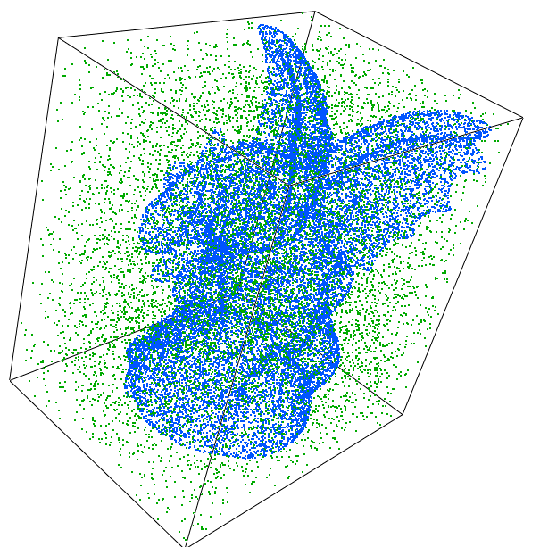
We took the gargoyle data set (Surface) from aim@shape, and generated the same number of random points in the bbox of the gargoyle (Random). We then consider three scenarios as data/queries. The data set contains 800K points. For each query point we compute the K=10,20,30 closest points, with the default splitter and for the bucket size 10 (default) and 20.
The results were produced with the release 5.1 of CGAL, on an Intel i7 2.3 Ghz laptop with 16 GB RAM, compiled with CLang++ 6 with the O3 option.
The values are the average of ten tests each. We show timings in seconds for both the building of the tree and the queries.
| k | bucket size | Surface Build | Random Build | Surface/Surface | Surface/Random | Random/Random |
|---|---|---|---|---|---|---|
| 10 | 10 | 0.17 | 0.31 | 1.13 | 15.35 | 3.40 |
| 10 | 20 | 0.14 | 0.28 | 1.09 | 12.28 | 3.00 |
| 20 | 10 | (see above) | (see above) | 1.88 | 18.25 | 5.39 |
| 20 | 20 | (see above) | (see above) | 1.81 | 14.99 | 4.51 |
| 30 | 10 | (see above) | (see above) | 2.87 | 22.62 | 7.07 |
| 30 | 20 | (see above) | (see above) | 2.66 | 18.39 | 5.68 |
The same experiment is done using the parallel version of the tree building algorithm, and performing the queries in parallel too:
| k | bucket size | Surface Build | Random Build | Surface/Surface | Surface/Random | Random/Random |
|---|---|---|---|---|---|---|
| 10 | 10 | 0.07 | 0.12 | 0.24 | 3.52 | 0.66 |
| 10 | 20 | 0.06 | 0.12 | 0.22 | 2.87 | 0.57 |
| 20 | 10 | (see above) | (see above) | 0.41 | 4.28 | 1.02 |
| 20 | 20 | (see above) | (see above) | 0.38 | 3.43 | 0.88 |
| 30 | 10 | (see above) | (see above) | 0.58 | 4.90 | 1.44 |
| 30 | 20 | (see above) | (see above) | 0.60 | 4.28 | 1.28 |
Bentley [3] introduced the kd tree as a generalization of the binary search tree in higher dimensions. kd trees hierarchically decompose space into a relatively small number of rectangles such that no rectangle contains too many input objects. For our purposes, a rectangle in real d dimensional space, \( \mathbb{R}^d\), is the product of d closed intervals on the coordinate axes. kd trees are obtained by partitioning point sets in \( \mathbb{R}^d\) using (d-1)-dimensional hyperplanes. Each node in the tree is split into two children by one such separating hyperplane. Several splitting rules (see Section Splitting Rules can be used to compute a separating (d-1)-dimensional hyperplane.
Each internal node of the kd tree is associated with a rectangle and a hyperplane orthogonal to one of the coordinate axis, which splits the rectangle into two parts. Therefore, such a hyperplane, defined by a splitting dimension and a splitting value, is called a separator. These two parts are then associated with the two child nodes in the tree. The process of partitioning space continues until the number of data points in the rectangle falls below some given threshold. The rectangles associated with the leaf nodes are called buckets, and they define a subdivision of the space into rectangles. Data points are only stored in the leaf nodes of the tree, not in the internal nodes.
Friedmann, Bentley and Finkel [4] described the standard search algorithm to find the kth nearest neighbor by searching a kd tree recursively.
When encountering a node of the tree, the algorithm first visits the child that is closest to the query point. On return, if the rectangle containing the other child lies within 1/ (1+ \( \epsilon\)) times the distance to the kth nearest neighbors so far, then the other child is visited recursively. Priority search [2] visits the nodes in increasing order of distance from the queue with help of a priority queue. The search stops when the distance of the query point to the nearest nodes exceeds the distance to the nearest point found with a factor 1/ (1+ \( \epsilon\)). Priority search supports next neighbor search, standard search does not.
In order to speed-up the internal distance computations in nearest neighbor searching in high dimensional space, the approximate searching package supports orthogonal distance computation. Orthogonal distance computation implements the efficient incremental distance computation technique introduced by Arya and Mount [1]. This technique works only for neighbor queries with query items represented as points and with a quadratic form distance, defined by \( d_A(x,y)= (x-y)A(x-y)^T\), where the matrix \( A\) is positive definite, i.e. \( d_A(x,y) \geq 0\). An important class of quadratic form distances are weighted Minkowski distances. Given a parameter \( p>0\) and parameters \( w_i \geq 0, 0 < i \leq d\), the weighted Minkowski distance is defined by \( l_p(w)(r,q)= ({\Sigma_{i=1}^{i=d} \, w_i(r_i-q_i)^p})^{1/p}\) for \( 0 < p <\infty\) and defined by \( l_{\infty}(w)(r,q)=max \{w_i |r_i-q_i| \mid 1 \leq i \leq d\}\). The Manhattan distance ( \( p=1\), \( w_i=1\)) and the Euclidean distance ( \( p=2\), \( w_i=1\)) are examples of a weighted Minkowski metric.
To speed up distance computations also transformed distances are used instead of the distance itself. For instance for the Euclidean distance, to avoid the expensive computation of square roots, squared distances are used instead of the Euclidean distance itself.
Not storing the points coordinates inside the tree usually generates a lot of cache misses, leading to non-optimal performance. This is the case for example when indices are stored inside the tree, or to a lesser extent when the points coordinates are stored in a dynamically allocated array (e.g., Epick_d with dynamic dimension) — we says "to a lesser extent" because the points are re-created by the kd-tree in a cache-friendly order after its construction, so the coordinates are more likely to be stored in a near-optimal order on the heap. In this case, the EnablePointsCache template parameter of the Kd_tree class can be set to Tag_true. The points coordinates will then be cached in an optimal way. This will increase memory consumption but provide better search performance. See also the GeneralDistance and FuzzyQueryItem concepts for additional requirements when using such a cache.
The initial implementation of this package was done by Hans Tangelder and Andreas Fabri. It was optimized in speed and memory consumption by Markus Overtheil during an internship at GeometryFactory in 2014. The EnablePointsCache feature was introduced by Clément Jamin in 2019. The parallel kd tree build function was introduced by Simon Giraudot in 2020.
 1.8.13